Variance and standard deviation

Abstract

Variance and standard deviation built from the ground up: the genesis of the concept of spread, why the mean is not enough, the derivation of the formula step by step (why square), variance as the average area of squares of deviations, the standard deviation and its interpretation, population versus sample and Bessel's correction with justification, Chebyshev's inequality, covariance and the covariance ellipse, and the generalisation to ℝⁿ. Every concept and every example with its own figure.

The mean tells us where the “centre” of the data lies, but says nothing about how widely the values are spread around it. This gap is filled by variance and standard deviation — the most important measures of variability in all of statistics and econometrics. This chapter derives them from the ground up: from the question of why the mean is not enough, through the construction of the formula step by step, up to covariance and the generalisation to the space $\mathbb{R}^n$. Every concept and every example is given its own figure.

Why the mean is not enough

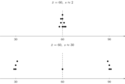
Consider two classes taking the same test. Both achieved a mean of $60$ points, yet their scores are distributed quite differently: in the first everyone scored $58$–$62$, while in the second half scored $30$ and half scored $90$. The mean is identical, though the situations are extremely different. We need a measure of how far the values deviate from the centre.

Two sets with the same mean and different spread — The same means, different spread. The upper set is concentrated around the mean $60$ (small deviation, $s\approx 2$), the lower one is spread to the extremes (large deviation, $s\approx 30$). The mean cannot tell them apart; the standard deviation can.

The genesis of measures of spread

The idea of measuring spread grew out of astronomy and the theory of errors at the turn of the eighteenth and nineteenth centuries, when Gauss and Legendre analysed the deviations of measurements from a mean value (see the least squares method). The term standard deviation itself was introduced by Karl Pearson in 1893, and the name variance by Ronald Fisher in 1918, making it the foundation of the analysis of variance (ANOVA). The common thread was the question of how to express, with a single number, the typical distance of observations from the mean — and it is precisely this number that we now construct.

Deriving the formula step by step

The natural idea is to average the distances of the observations from the mean. The first attempt, however, runs into an obstacle that must be circumvented.

Proof

Where the variance formula comes from

Deviation. For each observation we compute the deviation from the mean $d_i=x_i-\bar{x}$ — it says how far and in which direction the value lies.
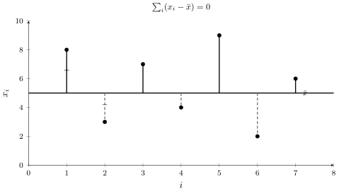
The obstacle. The sum of the deviations is always zero: $\sum_i(x_i-\bar{x})=\sum_i x_i-n\bar{x}=n\bar{x}-n\bar{x}=0$. The positives cancel the negatives, so the “mean deviation” would be a useless zero.
The fix — squaring. We square each deviation: $d_i^2=(x_i-\bar{x})^2\ge 0$. The squares do not cancel, and they additionally weight large deviations more heavily.
Variance. We average the squared deviations: $$\sigma^2=\frac{1}{n}\sum_{i=1}^{n}(x_i-\bar{x})^2.$$
Back to units. The variance is expressed in squared units (e.g. “dollars squared”), which hinders interpretation. The square root restores the original units — this is the standard deviation: $$\sigma=\sqrt{\sigma^2}=\sqrt{\frac{1}{n}\sum_{i=1}^{n}(x_i-\bar{x})^2}.$$

∎

The second step — the vanishing of the sum of deviations — is the heart of the whole construction. This is why we square rather than simply sum.

Positive and negative deviations from the mean cancelling to zero — The sum of deviations from the mean is always zero: the positive deviations (solid lines, above $\bar{x}$) exactly balance the negative ones (dashed lines, below). This is why we use their squares to measure spread, not the deviations themselves.

Variance as the average area of squares

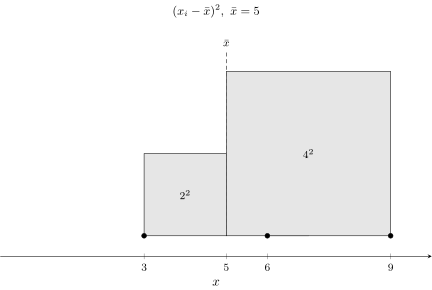
The word “square” is to be understood literally: each deviation $(x_i-\bar{x})$ determines a square with side equal to that distance, and its area is $(x_i-\bar{x})^2$. The variance is the average area of these squares — a geometric interpretation that explains why large deviations weigh so heavily (the area grows with the square of the side).

Squares of deviations as areas — a geometric interpretation of variance — Each deviation from the mean $\bar{x}=5$ spans a square of area $(x_i-\bar{x})^2$. An observation $4$ away gives a square of area $16$ — four times larger than for a deviation of $2$. The variance is the average area of such squares.

A numerical example

For the set $2,4,4,4,5,5,7,9$ we have $n=8$ and $\bar{x}=\tfrac{40}{8}=5$. The deviations are $-3,-1,-1,-1,0,0,2,4$, and their squares $9,1,1,1,0,0,4,16$ sum to $32$. Hence the population variance

$$ \sigma^2=\frac{32}{8}=4,\qquad \sigma=\sqrt{4}=2. $$

The typical value thus lies about $2$ units from the mean.

Interpreting the standard deviation

How to read the standard deviation.

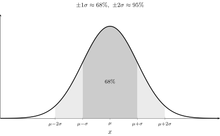
The standard deviation is the typical distance of an observation from the mean, expressed in the same units as the data. If wages have a mean of $5000$ and $\sigma=800$, then a “typical” person earns about $800$ above or below the mean. For data shaped like the normal distribution, about $68\%$ of observations fall in the interval $\mu\pm\sigma$, and about $95\%$ in $\mu\pm 2\sigma$.

Intervals plus or minus one and two standard deviations — The $\pm\sigma$ rule for a distribution close to normal: about $68\%$ of observations lie in $\mu\pm\sigma$ (dark area), and about $95\%$ in $\mu\pm 2\sigma$. The standard deviation sets the natural scale of spread.

But what if the distribution is not normal? Then a theorem that holds for any distribution helps.

Theorem

Chebyshev's inequality

For any distribution with finite variance, the proportion of observations more than $k$ standard deviations away from the mean does not exceed $\tfrac{1}{k^2}$:

$$ P\big(|X-\mu|\ge k\sigma\big)\le\frac{1}{k^2}. $$

Hence at least $1-\tfrac{1}{k^2}$ of the mass lies in the interval $\mu\pm k\sigma$ — e.g. at least $75\%$ in $\mu\pm2\sigma$ and $\approx 89\%$ in $\mu\pm3\sigma$, regardless of the shape of the distribution.

Population versus sample: Bessel’s correction

A subtlety arises here that is a frequent source of mistakes. The formula depends on whether we have the whole population or merely a sample of it:

$$ \sigma^2=\frac{1}{n}\sum(x_i-\bar{x})^2\ \text{(population)},\qquad s^2=\frac{1}{n-1}\sum(x_i-\bar{x})^2\ \text{(sample)}. $$

Where the divisor $n-1$ comes from (Bessel’s correction).

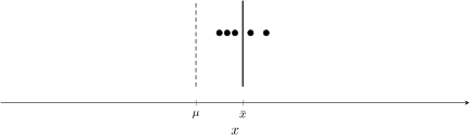
When computing the sample variance, we measure the deviations against the estimated mean $\bar{x}$, not the true population mean $\mu$. A sample always lies closer to its own mean than to the true one, so the sum of squared deviations is systematically underestimated. Dividing by $n-1$ rather than $n$ corrects this bias and yields an unbiased estimator. For our example the sample variance is $s^2=\tfrac{32}{7}\approx 4.57$, and $s\approx 2.14$ — slightly more than the population value of $4$. For large $n$ the difference vanishes.

The sample mean lying closer to the data than the true population mean — The mechanism of Bessel’s correction: the sample (points) clusters around its own mean $\bar{x}$, which usually lies closer to the data than the unknown true mean $\mu$. Deviations measured against $\bar{x}$ are therefore too small — the divisor $n-1$ makes up for it.

The most common coding mistake.

In R the functions var() and sd() divide by $n-1$ (sample), whereas in NumPy np.var() and np.std() divide by $n$ (population) by default. If results from R and Python differ, the cause is almost always this discrepancy — in NumPy one must add the argument ddof=1 to obtain the sample variance.

From variance to covariance

Variance measures the spread of a single variable. When there are several variables, we are interested in whether they vary together — this is measured by covariance:

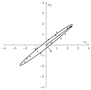
$$ \mathrm{Cov}(x,y)=\frac{1}{n}\sum_{i=1}^{n}(x_i-\bar{x})(y_i-\bar{y}). $$

Covariance is a natural generalisation of variance (for $y=x$ it reduces to $\sigma^2$) and underlies correlation and the regression slope, where $b_1=\mathrm{Cov}(x,y)/\mathrm{Var}(x)$. Geometrically, the spread of two variables is represented by the covariance ellipse: its longer axis points in the direction of greatest variability, and its shape reflects the strength of the co-variation.

Covariance ellipse with principal axes of spread — The covariance ellipse of two variables: the cloud of observations stretches along one direction. The longer arrow is the axis of greatest spread, the shorter one the direction of least spread. The variance in each direction is the length of the corresponding semi-axis.

Generalisation to the space $\mathbb{R}^n$

For many variables the variances and covariances are collected into a covariance matrix — a symmetric array in which the diagonal holds the variances of the individual variables and the off-diagonal entries their covariances. This matrix fully describes the spread of the data cloud in the space $\mathbb{R}^n$.

Covariance ellipsoid in three-dimensional space — The covariance ellipsoid in the space $\mathbb{R}^3$: the spread of three variables has the shape of a solid with three semi-axes whose lengths are the variances along the principal directions. This is the three-dimensional counterpart of the covariance ellipse.

The covariance matrix and the fourth dimension.

The directions along which the data cloud stretches most are the eigenvectors of the covariance matrix, and the corresponding variances are its eigenvalues. In $\mathbb{R}^2$ the spread has the shape of an ellipse, in $\mathbb{R}^3$ an ellipsoid, and in $\mathbb{R}^4$ and higher a solid that cannot be drawn but is fully described by the covariance matrix. A four-dimensional spread is analysed “layer by layer,” projecting it onto pairs and triples of variables. On this idea — reducing a multidimensional spread to a few directions of greatest variance — rests principal component analysis (PCA).

Application — case study: stock volatility (risk)

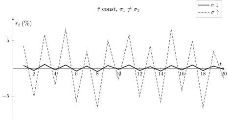
In finance the standard deviation of returns is called volatility and is the basic measure of risk. Consider two companies with the same mean daily return close to zero but different spread: a stable company with daily $\sigma_1=0.5\%$ and a volatile one with $\sigma_2=5\%$. Although on average they earn the same, the second is ten times riskier.

Daily volatility is converted to annual by the square-root-of-time rule (with about $252$ trading days):

$$ \sigma_{\text{year}}=\sigma_{\text{day}}\sqrt{252}. $$

For the stable company $\sigma_{\text{year}}=0.5\%\cdot\sqrt{252}\approx 7.9\%$, for the volatile one $5\%\cdot\sqrt{252}\approx 79\%$. The $\sqrt{252}$ rule follows from the additivity of the variance of independent increments: the variance of a sum over $252$ days is $252\sigma_{\text{day}}^2$, so the deviation grows as the square root.

Two return series with different volatility — Two companies with the same mean return but different standard deviation. The upper series (small $\sigma$) is stable, the lower one (large $\sigma$) is highly volatile. The variance of returns is a measure of risk.

This case study shows that variance is not merely a statistical abstraction: it is a numerical measure of risk underlying portfolio theory, option pricing, and market risk management.