The central limit theorem

Abstract

The central limit theorem built from the ground up: genesis (the Galton board, the de Moivre–Laplace theorem, Lindeberg and Lévy), the law of large numbers, the statement of the theorem, an illustration of the convergence of the distribution of the mean to the normal regardless of the population, the standard error and the square-root-of-n rule, the multivariate CLT in 3D, the significance for econometric inference, and verification by simulation. Every concept and every example with its own figure.

The central limit theorem (CLT) explains why the normal distribution appears almost everywhere — and why hypothesis tests and confidence intervals work at all. Its content is surprising: the sample mean has an approximately normal distribution regardless of the shape of the distribution we sample from. This chapter builds the theorem from the ground up: from its genesis and the law of large numbers, through the precise statement and its illustration, up to the multivariate generalisation and the significance for econometrics. Every concept and every example is given its own figure.

Genesis

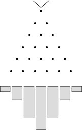
The first version of the theorem was proved by Abraham de Moivre (1733) and Pierre-Simon Laplace: the distribution of the number of successes in many Bernoulli trials — the binomial — tends to the normal distribution. In the nineteenth and twentieth centuries Pafnuty Chebyshev, Aleksandr Lyapunov, and Jarl Lindeberg and Paul Lévy generalised it to sums of arbitrary independent variables with finite variance, giving the theorem its modern form. A tangible illustration is the Galton board (quincunx): balls falling through a grid of pegs, bouncing randomly left or right in each row, collect at the bottom into a bell shape — because the final position of each ball is a sum of many independent deflections.

Galton board — balls forming a bell-shaped distribution — The Galton board: a ball passes through successive rows of pegs, bouncing randomly left or right at each. The final bin is the sum of these random steps, so the bars line up into a bell curve. A mechanical illustration of the central limit theorem.

The law of large numbers

Before stating the CLT, it is worth separating it from a kindred but weaker theorem. The law of large numbers says that the sample mean converges to the true population mean as the sample size grows:

$$ \bar{X}_n\xrightarrow{n\to\infty}\mu. $$

This is the guarantee that averaging “works” — a larger sample gives an ever more accurate estimate of the mean.

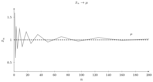
Running mean converging to the true mean — The law of large numbers: the running mean $\bar{x}_n$ (the broken line) fluctuates strongly at first, but as the number of observations grows it settles down and converges to the true mean $\mu$ (the dashed line).

The law of large numbers, however, says only where the mean converges. The central limit theorem goes further — it describes the shape of its fluctuations around that limit.

The statement of the theorem

Theorem

The central limit theorem (Lindeberg–Lévy)

If $X_1,X_2,\dots$ are independent, identically distributed with mean $\mu$ and finite variance $\sigma^2$, then the distribution of the sample mean tends to the normal:

$$ \bar{X}_n\;\xrightarrow{\;n\to\infty\;}\;\mathcal{N}\!\Big(\mu,\frac{\sigma^2}{n}\Big), $$

regardless of the shape of the original distribution. Equivalently, the standardised sum $\tfrac{\sqrt{n}(\bar{X}_n-\mu)}{\sigma}$ tends to $\mathcal{N}(0,1)$.

Illustration: a bell from any distribution

Let us illustrate the theorem on an extremely asymmetric distribution — the exponential. The population is strongly right-skewed, yet the distribution of sample means becomes ever more bell-shaped and ever narrower as $n$ grows.

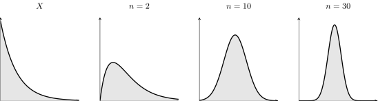
A skewed distribution and distributions of means becoming a bell as n grows — The central limit theorem in action. The population (far left) is strongly skewed (exponential). The distribution of sample means for $n=2$ is still skewed, for $n=10$ nearly symmetric, and for $n=30$ already a bell curve — ever narrower, because concentrated around $\mu$.

As $n$ increases, two things happen at once: the shape becomes normal (even if the population was not), and the width decreases (the means cluster ever more tightly around the true $\mu$).

Universality

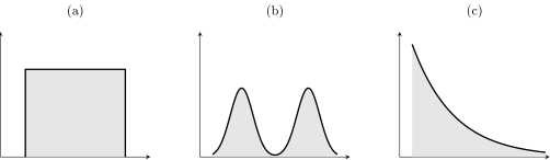
The most remarkable feature of the CLT is its universality: the starting point does not matter. Whether the population is uniform, bimodal, or skewed, the distribution of the mean of a sufficiently large sample tends to the same bell curve.

Three different populations leading to the same normal distribution of means — Three completely different populations: (a) uniform (flat), (b) bimodal (two peaks), (c) skewed. Despite their different shapes, the distribution of the mean of a large sample tends to the same normal distribution for each — this is the universality of the CLT.

The standard error and the $\sqrt{n}$ rule

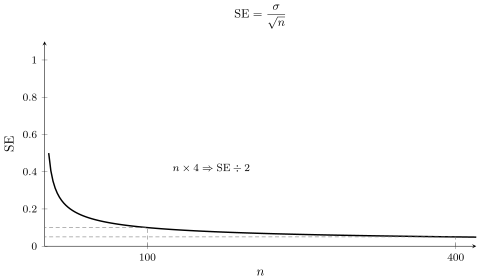
The standard deviation of the distribution of the mean has its own name — the standard error:

$$ \mathrm{SE}=\frac{\sigma}{\sqrt{n}}. $$

It decreases as the inverse of the square root of the sample size, which has important practical consequences.

What the $\sqrt{n}$ rule says.

To halve the error of an estimate of the mean, it is not enough to double the data — one needs four times as much. Precision grows as the square root of the sample size, not linearly. This is why the final refinements in research cost disproportionately much.

Standard error decreasing as one over the square root of n — The standard error decreases as $\sigma/\sqrt{n}$ — quickly at first, then ever more slowly. Going from $n=100$ to $n=400$ (a fourfold increase in sample size) halves the error exactly.

The multivariate limit theorem

The CLT generalises to random vectors: the sample mean of vectors (with a common mean and covariance matrix) tends to the multivariate normal distribution. A sum of many independent vectors, suitably rescaled, forms a multidimensional bell.

A two-dimensional bell as the limit of a sum of random vectors — The multivariate CLT: the mean (sum) of many independent random vectors tends to a multivariate normal distribution — here a two-dimensional bell. It is thanks to this that the vector of OLS estimators has an approximately normal distribution in large samples.

The CLT in $\mathbb{R}^n$ and estimation.

OLS estimators are weighted sums of observations, so by the multivariate CLT they have, in large samples, an approximately multivariate normal distribution — with a mean vector equal to the true parameters and a covariance matrix determining their precision. This is why one can test the significance of coefficients and build confidence intervals even when the error term is not exactly normal: the CLT “supplies” normality asymptotically. The geometry works in any dimension $\mathbb{R}^n$, although beyond three dimensions the bell cannot be drawn.

Significance for econometrics

Confidence intervals for the mean work because $\bar{X}$ is approximately normal — hence the formula $\bar{x}\pm 1.96\cdot\mathrm{SE}$.
$t$ and $z$ tests assume the normality of the test statistic, which the CLT provides for a sufficiently large sample.
OLS estimators are sums, so they are asymptotically normal — the foundation of significance testing.

Required sample size.

A practical rule: $n\ge 30$ usually suffices. But for a strongly skewed or heavy-tailed population, more observations are needed — the farther the original distribution from normal, the larger the $n$ required for the mean to have time to “normalise.”

Verification by simulation

The simplest empirical proof is a simulation: we repeatedly draw samples from the extremely skewed exponential distribution, compute their means, and look at the histogram.

# R — draw from a strongly skewed exponential distribution and average
set.seed(1)
means <- replicate(10000, mean(rexp(30, rate = 1)))
hist(means, breaks = 40)   # despite the skewed population — a bell curve

# Python
import numpy as np
means = [np.mean(np.random.exponential(1, 30)) for _ in range(10000)]
# histogram(means) -> a bell curve

Changing the sample size from $30$ to $2$ or $100$ lets one observe how the shape, with growing $n$, approaches a perfect bell.

Application — case study: an election poll and the margin of error

The central limit theorem explains why a poll of $1000$ people can estimate the support of an entire society. Let the true support for a party be $p$. The proportion $\hat{p}$ in a random sample of $n$ people is a mean of zeros and ones, so by the CLT it has an approximately normal distribution with standard error $\sqrt{p(1-p)/n}$. The margin of error at a $95\%$ confidence level is

$$ \text{MoE}=1.96\sqrt{\frac{p(1-p)}{n}}. $$

For $n=1000$ and the conservative assumption $p=0.5$ (maximising the variance):

$$ \text{MoE}=1.96\sqrt{\frac{0.25}{1000}}\approx 0.031=\pm 3.1\ \text{percentage points.} $$

Hence the famous “$\pm 3$ percentage points” in polling reports. To halve the margin (to $\pm 1.5$ pts), the $\sqrt{n}$ rule requires a fourfold larger sample — $4000$ people.

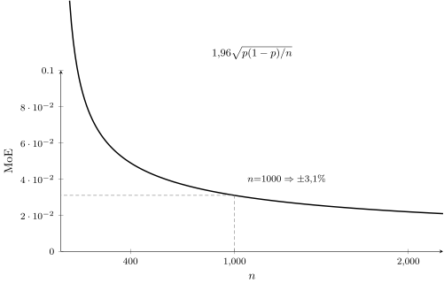
A poll's margin of error decreasing with sample size — The poll’s margin of error decreases as $1.96\sqrt{p(1-p)/n}$. For $n=1000$ it is about $\pm 3.1$ percentage points; further increasing the sample improves precision ever more slowly (the $\sqrt{n}$ rule).

This case study shows that the CLT is the foundation of all polling and survey practice: without it we could neither state a margin of error nor justify why a sample of about a thousand suffices to gauge the opinion of millions.