Descriptive statistics

Abstract

Descriptive statistics built from the ground up: genesis (Graunt, Quetelet, Galton, Pearson), types of variables, measures of location (the mean as a balance point, median, mode) with an analysis of outliers, measures of variability (variance, standard deviation, coefficient of variation), quantiles and the box plot, skewness and kurtosis, the correlation coefficient, standardisation, and multivariate data in ℝⁿ. Every concept and every example with its own figure.

Descriptive statistics is the art of summarising data: replacing thousands of numbers with a few quantities that capture their location, spread, and shape. It is the starting point of every econometric analysis — before building a model, we must know the data. This chapter builds the apparatus of descriptive statistics from its genesis, through measures of location and variability, up to the description of multivariate data in the space $\mathbb{R}^n$. Every concept and every example is given its own figure.

The genesis of descriptive statistics

Statistics was born of the need to govern a state — the very name derives from the Latin status. In 1662 the London merchant John Graunt published an analysis of the “bills of mortality,” tabulating the numbers of deaths by cause and by season; it was the first attempt to extract regularities from raw numerical data. In the nineteenth century the Belgian scholar Adolphe Quetelet introduced the notion of the average man (l’homme moyen), applying the mean to describe human characteristics and making the mean the central concept of social statistics. Toward the end of the nineteenth century Francis Galton and Karl Pearson built the apparatus of correlation and regression, giving descriptive statistics its modern form — and opening the road to econometrics. We begin with the distinction that precedes all computation: the types of data.

Types of variables

The choice of measure depends on the type of data we work with.

Type	Example	Meaningful measures
Nominal	sex, region	mode, frequency
Ordinal	rating (1–5), satisfaction level	median, quantiles
Quantitative (interval, ratio)	GDP, income, price	mean, standard deviation, correlation

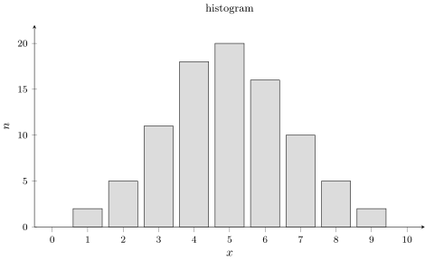
In econometrics we work mainly with quantitative variables, for which the full statistical apparatus is available. The first step in describing them is usually a histogram — a chart showing how often the values fall into successive intervals.

Histogram — counts of observations in successive intervals — A histogram divides the range of the data into intervals and shows the count of each. From its shape we read the location (where the mass concentrates), the spread (how wide the distribution is), and the symmetry.

Measures of location

Measures of location indicate the “centre” of the data — the typical value around which the observations cluster.

The arithmetic mean

Definition

Arithmetic mean

The arithmetic mean of a set $x_1,\dots,x_n$ is

$$ \bar{x}=\frac{1}{n}\sum_{i=1}^{n}x_i=\frac{x_1+x_2+\dots+x_n}{n}. $$

It takes every observation into account and is the point about which the sum of deviations is zero: $\sum_i(x_i-\bar{x})=0$.

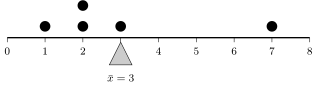
The vanishing of the sum of deviations has a vivid physical interpretation: the mean is the balance point of the data. If the observations were weights placed on a weightless beam, the beam would balance exactly at the point $\bar{x}$.

The mean as the balance point of a beam with weights — The mean as a balance point. The observations $1,2,2,3,7$ are weights on a beam; a support placed at $\bar{x}=3$ keeps it in balance, because the sums of moments on both sides are equal. Hence $\sum_i(x_i-\bar{x})=0$.

Median and mode: resistance to outliers

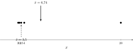
A weakness of the mean is its sensitivity to outliers. The median — the middle value after ordering the data — is resistant to them, and the mode is the most frequent value. Consider the earnings of five people (in thousands): $3.0,\ 3.2,\ 3.5,\ 4.0,\ 20.0$. The mean is

$$ \bar{x}=\frac{3.0+3.2+3.5+4.0+20.0}{5}=6.74, $$

while the median is $3.5$. The mean, inflated by a single high salary, poorly describes the “typical” employee — the median is fairer here.

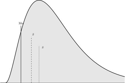
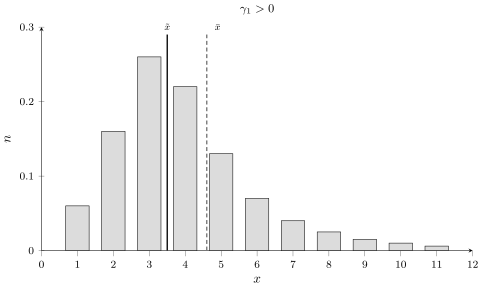
An outlier dragging the mean, the median stable — Five earnings on a number line. A single outlier ($20$k) drags the mean $\bar{x}=6.74$ far to the right, while the median $\tilde{x}=3.5$ stays with the main group. For skewed data the median is the more appropriate measure of location.

When the distribution is asymmetric, the three measures of location diverge: the mode lies at the peak, the median at the middle of the mass, and the mean is dragged toward the long tail.

Mean, median, and mode in a skewed distribution — In a skewed distribution the mode (Mo), median ($\tilde{x}$), and mean ($\bar{x}$) diverge. The long tail (e.g. a few very wealthy people) drags the mean toward it — which is why for skewed data the median is fairer.

Measures of variability

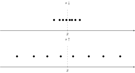
Location alone is not enough — two sets with the same mean can differ drastically in spread.

Variance and standard deviation

Definition

Sample variance and standard deviation

The sample variance is the mean squared deviation from the mean:

$$ s^2=\frac{1}{n-1}\sum_{i=1}^{n}(x_i-\bar{x})^2, $$

and the standard deviation is its square root $s=\sqrt{s^2}$. Dividing by $n-1$ (rather than $n$) gives an unbiased estimator of the population variance — the details are explained in the chapter on variance and deviation.

The variance begins with the deviations $x_i-\bar{x}$ — the distances of each observation from the mean. So that positive and negative deviations do not cancel, we square them and then average.

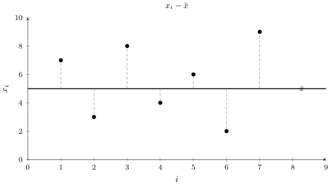
Deviations of observations from the mean — Deviations from the mean: dashed lines connect each observation to the level of the mean $\bar{x}$. The variance is the averaged square of these distances — the longer the deviations, the larger the variance.

The standard deviation is expressed in the same units as the data, so it is easy to interpret: for $\bar{x}=30$k and $s=5$k, most observations fall in the range $25$–$35$k.

Small and large variance — spread of data around the mean — Both sets have the same mean but different spread: on the left, concentrated data (small $s$); on the right, dispersed data (large $s$). Variance and standard deviation measure precisely this difference.

The coefficient of variation

To compare the variability of quantities expressed in different units or on different scales, we use the coefficient of variation — the standard deviation relative to the mean:

$$ CV=\frac{s}{\bar{x}}\cdot 100\%. $$

It lets us state that, for example, apartment prices (in hundreds of thousands) and bread prices (in single units) have comparable relative variability, despite incomparable units.

Quantiles and the box plot

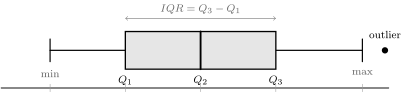
Quantiles divide ordered data into equal parts. The most important are the quartiles: $Q_1$ (25th percentile), $Q_2$ (median), and $Q_3$ (75th percentile). The difference $IQR=Q_3-Q_1$ — the interquartile range — covers the middle 50% of the observations and is a measure of spread resistant to outliers.

The box plot summarises these quantities in a single figure, making it an excellent tool for comparing distributions.

Box plot — quartiles, IQR, whiskers, and an outlier — The box plot: the “box” covers the middle 50% of the data (from $Q_1$ to $Q_3$), the line inside is the median, the whiskers reach the extreme typical values, and a point beyond them is an outlier.

The shape of a distribution: skewness and kurtosis

After location and spread, the third feature of a distribution is its shape, described by higher-order moments.

Skewness

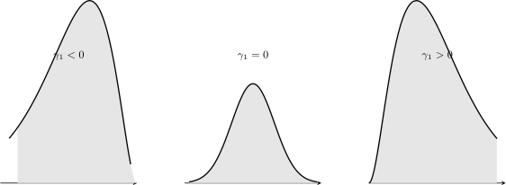
Skewness measures the asymmetry of a distribution and is based on the third power of the deviations:

$$ \gamma_1=\frac{\tfrac{1}{n}\sum(x_i-\bar{x})^3}{s^3}. $$

A positive value means a long tail on the right (right skew), negative means on the left, and zero means symmetry. Income data are typically strongly right-skewed: a few very wealthy people form a long tail.

Left-skewed, symmetric, and right-skewed distributions — Skewness indicates which way a distribution “leans”: $\gamma_1<0$ (tail to the left), $\gamma_1=0$ (symmetry), and $\gamma_1>0$ (tail to the right, typical of incomes).

Kurtosis

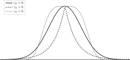
Kurtosis measures the “heaviness of the tails” and the peakedness relative to the normal distribution, based on the fourth power of the deviations:

$$ \gamma_2=\frac{\tfrac{1}{n}\sum(x_i-\bar{x})^4}{s^4}-3. $$

A positive value ($\gamma_2\gt 0$, a leptokurtic distribution) means a sharper peak and heavier tails — more extreme events, which is of key importance in financial risk analysis.

Kurtosis — leptokurtic, normal, and platykurtic distributions — Kurtosis describes the peakedness and the heaviness of the tails: $\gamma_2>0$ (leptokurtic — sharp, heavy tails, more extreme events), $\gamma_2=0$ (normal), and $\gamma_2<0$ (platykurtic — flattened).

The correlation coefficient

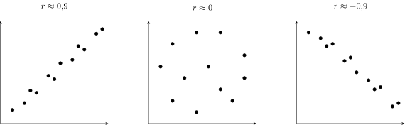
When we observe pairs of quantities, we are interested in whether they vary together. The Pearson correlation coefficient measures the strength and direction of a linear relationship:

$$ r=\frac{\sum_{i=1}^{n}(x_i-\bar{x})(y_i-\bar{y})}{(n-1)\,s_x s_y}\in[-1,1]. $$

A value $r=1$ means a perfect increasing relationship, $r=-1$ a decreasing one, and $r=0$ no linear relationship. We develop the full theory of correlation in a separate chapter; here we merely note its role in describing data.

Scatter plots: positive, no, and negative correlation — The correlation coefficient $r$ measures the strength and direction of a linear relationship: positive ($r\approx 0.9$ — points line up increasing), none ($r\approx 0$ — a cloud), and negative ($r\approx -0.9$ — decreasing).

Correlation is not causation.

A high correlation between two variables does not prove that one influences the other. Both may depend on a common third variable (a confounder) or co-occur by chance. Distinguishing association from causation is the central problem of econometrics.

Standardisation

To compare observations from different distributions or expressed in different units, we transform them to a common scale.

Definition

Standardisation (the $z$-score)

Standardisation is the transformation

$$ z_i=\frac{x_i-\bar{x}}{s}, $$

which shifts the mean to zero and scales the standard deviation to one. A value $z=2$ means “two standard deviations above the mean,” regardless of the original units.

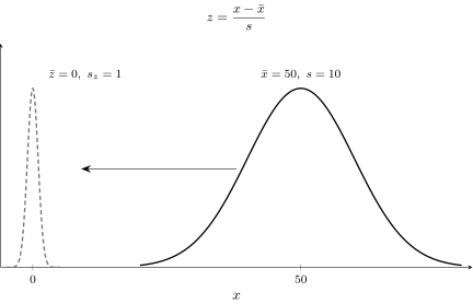
Standardisation of a distribution to mean zero and deviation one — Standardisation shifts the distribution so that the mean is $0$ and scales it so that the standard deviation is $1$. A wide distribution $\bar{x}=50,\ s=10$ becomes the narrow standard one $\bar{z}=0,\ s_z=1$ — the shape stays, only the scale and location change.

Standardisation is indispensable when comparing variables of different units or applying scale-sensitive methods (regularised regression, principal component analysis). The $z$-score is also a bridge to the normal distribution.

Multivariate data and the space $\mathbb{R}^n$

In econometrics we rarely describe a single variable. Usually each observation is a vector of many features at once — income, age, education, region. A set of $n$ observations described by $p$ features is a cloud of $n$ points in the space $\mathbb{R}^p$.

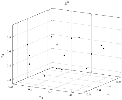
A cloud of data points in three-dimensional space — Data on three features as a cloud of points in the space $\mathbb{R}^3$: each observation is a point with coordinates $(x_1,x_2,x_3)$. Descriptive statistics (means, variances, correlations) summarise the location and shape of this cloud.

Describing a cloud in $\mathbb{R}^p$ and the fourth dimension.

For many features the means form a mean vector, and the variances and correlations a covariance matrix (see linear algebra). Geometrically the mean vector indicates the centre of the cloud, and the covariance matrix describes its shape and orientation — the directions of greatest spread are its eigenvectors. When there are four or more features, the cloud cannot be drawn, but the same quantities describe it completely. A four-dimensional cloud can be viewed “layer by layer” — by projecting it onto successive pairs or triples of features — and this is exactly how, projection by projection, multivariate data are analysed in practice.

Application — case study: the wage distribution

Descriptive statistics best reveals its value on wage data, which are typically strongly right-skewed. According to Polish official statistics (GUS), the average gross monthly wage is markedly higher than the median — because a small group of very high salaries inflates the mean. Take, for illustration: mean $\bar{x}\approx 8000$, median $\tilde{x}\approx 6600$, standard deviation $s\approx 4000$.

From these numbers we read the wage structure:

median $\lt$ mean confirms right skew ($\gamma_1\gt 0$): the “typical” worker earns less than the mean suggests;
the coefficient of variation $CV=\tfrac{s}{\bar{x}}=\tfrac{4000}{8000}=50\%$ indicates large wage dispersion;
the median is the fairer description of a “typical” wage — which is why official releases report both measures.

Right-skewed wage distribution: median below the mean — The wage distribution is right-skewed: most workers earn below the mean, and the long tail of high salaries drags the mean $\bar{x}$ to the right of the median $\tilde{x}$. Hence for wages the median better describes the “typical” value.

This case study illustrates a practical rule: the choice of measure must fit the shape of the data. For skewed distributions — and incomes, property prices, and firm revenues are such — the mean can mislead, and a true picture emerges only from the median, quantiles, and skewness measures together.

Descriptive statistics

The genesis of descriptive statistics

Types of variables

Measures of location

The arithmetic mean

Median and mode: resistance to outliers

Measures of variability

Variance and standard deviation

The coefficient of variation

Quantiles and the box plot

The shape of a distribution: skewness and kurtosis

Skewness

Kurtosis

The correlation coefficient

Standardisation

Multivariate data and the space $\mathbb{R}^n$

Application — case study: the wage distribution

Further reading

Summary