Probability distributions
Probability distributions built from the ground up: the genesis of probability theory, discrete and continuous random variables, the density function and the cumulative distribution function, the normal distribution, Student's t-distribution and its heavy tails, the chi-square distribution as a sum of squared normal variables, the F-distribution, the relationships between distributions, applications in hypothesis testing, and the generalisation to ℝⁿ. Every concept and every example with its own figure.
A probability distribution describes which values of a random variable are possible and how probable they are. Four distributions — the normal, Student’s $t$, chi-square, and $F$ — form a single system on which all of statistical inference rests: hypothesis tests and confidence intervals. This chapter builds them from the ground up: from the genesis of probability theory, through the density function and the cumulative distribution function, up to the mutual relationships of the distributions and their generalisation to the space $\mathbb{R}^n$. Every concept and every example is given its own figure.
The genesis of probability theory
Probability theory was born of games of chance. In 1654 Blaise Pascal and Pierre de Fermat, solving the puzzle of the fair division of stakes in an interrupted game, laid its foundations. Over the following centuries it was developed by Jacob Bernoulli, de Moivre, Laplace, and Gauss, until in 1933 Andrey Kolmogorov gave the theory a rigorous axiomatic form. The distributions used in econometrics date from the early twentieth century, when attention turned to inference from samples: William Gosset (under the pseudonym “Student”) introduced the $t$-distribution in 1908, Karl Pearson developed the chi-square test, and Ronald Fisher the $F$-distribution and the analysis of variance. All three grow out of the normal distribution, with which — after introducing the basic notions — we begin their survey.
Random variables and distributions
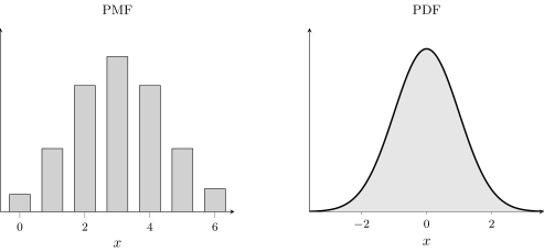
For a discrete variable the distribution is given by a probability mass function (PMF), assigning each value its probability. For a continuous variable a single value has probability zero, so the distribution is given by a density function (PDF), and probabilities are read as areas.
Density function and cumulative distribution function
The density function $f(x)$ satisfies $f(x)\ge 0$ and $\int_{-\infty}^{\infty}f(x)\,dx=1$, and probabilities are computed as integrals:
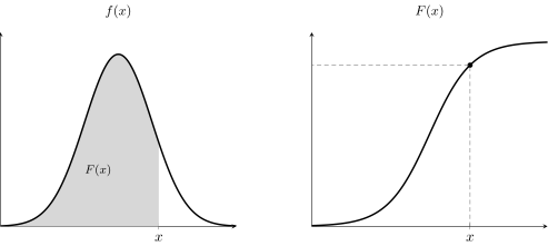
$$ P(a\le X\le b)=\int_a^b f(x)\,dx. $$The cumulative distribution function $F(x)=P(X\le x)=\int_{-\infty}^{x}f(t)\,dt$ is the accumulated probability — the area under the density to the left of $x$. By the fundamental theorem of calculus, $F'(x)=f(x)$.
The normal distribution $N(\mu,\sigma^2)$
The most important distribution in statistics is the normal distribution with density
$$ f(x)=\frac{1}{\sigma\sqrt{2\pi}}\exp\!\Big(-\frac{(x-\mu)^2}{2\sigma^2}\Big), $$where $\mu$ is the mean (the location of the peak) and $\sigma$ the standard deviation (the width). Every normal variable is reduced to the standard $N(0,1)$ by standardisation $Z=\tfrac{X-\mu}{\sigma}$. We develop the full theory of this distribution in a separate chapter; here we point to its role in inference.
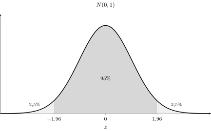
The boundary values follow from the $68$–$95$–$99.7$ rule: the interval $\mu\pm\sigma$ holds $68.3\%$ of the mass, $\mu\pm 2\sigma$ holds $95.4\%$, and $\mu\pm 3\sigma$ holds $99.7\%$. In hypothesis testing one most often uses the exact value $\mu\pm 1.96\sigma$, covering exactly $95\%$.
Student’s $t$-distribution
When the variance $\sigma^2$ is unknown and we estimate it from the data, the standardised mean has not a normal distribution but Student’s $t$:
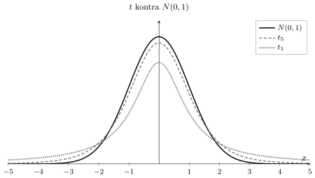
$$ t=\frac{\bar{X}-\mu_0}{s/\sqrt{n}}\sim t_{n-1}, $$where $s$ is the sample standard deviation and $n-1$ the number of degrees of freedom. The $t$-distribution resembles the normal but has heavier tails: the additional uncertainty from estimating $\sigma$ makes extreme values more probable. The more degrees of freedom, the closer to the normal — for $df\gt 30$ the difference is practically imperceptible.
In econometrics the $t$-distribution serves to test the significance of an individual regression coefficient: the statistic $t=\hat\beta_j/\mathrm{SE}(\hat\beta_j)$ has distribution $t_{n-k-1}$, and the hypothesis $H_0:\beta_j=0$ is rejected when $|t|$ exceeds the critical value.
The chi-square distribution $\chi^2_k$
The chi-square distribution with $k$ degrees of freedom is the distribution of the sum of squares of $k$ independent standard normal variables:
$$ \chi^2_k=Z_1^2+Z_2^2+\dots+Z_k^2,\qquad Z_i\sim N(0,1). $$It takes only nonnegative values, is right-skewed, and has expected value $k$ and variance $2k$.
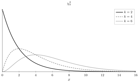
The origin of this distribution from a sum of squared normal variables can be seen geometrically. A pair of independent $Z_1,Z_2\sim N(0,1)$ has a joint density proportional to $e^{-(z_1^2+z_2^2)/2}$ — a two-dimensional bell. The squared distance of a point from the centre, $R^2=Z_1^2+Z_2^2$, is precisely a $\chi^2_2$ variable.

The chi-square distribution serves to test variance ($\tfrac{(n-1)s^2}{\sigma_0^2}\sim\chi^2_{n-1}$) and the independence of categorical variables (the test $\chi^2=\sum\tfrac{(O-E)^2}{E}$ on contingency tables).
The $F$-distribution
The $F$-distribution with degrees of freedom $k_1,k_2$ is the distribution of the ratio of two independent chi-square variables, each divided by its own degrees of freedom:
$$ F=\frac{\chi^2_{k_1}/k_1}{\chi^2_{k_2}/k_2}\sim F_{k_1,k_2}. $$It takes nonnegative values and is right-skewed.
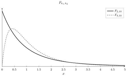
The $F$-distribution serves to test the joint significance of several regression coefficients at once ($H_0:\beta_1=\dots=\beta_k=0$) and linear restrictions (the Wald test). It compares the improvement in fit per variable with the unexplained variance per observation.
Relationships between the distributions
The four distributions form a single coherent system, all of it growing out of the normal distribution.
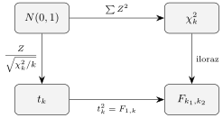
Distributions in $\mathbb{R}^n$ and inference.
All these distributions describe functions of a sample — quantities computed from $n$ observations, i.e. from a point in the space $\mathbb{R}^n$. The sum of squared residuals is the squared length of the residual vector in $\mathbb{R}^n$, and its distribution is chi-square with degrees of freedom equal to the dimension of the residual subspace. The geometry of the orthogonal projection from linear algebra thus explains where degrees of freedom come from: they are the dimensions of the perpendicular subspaces into which the observation vector decomposes. Four-dimensional and higher-dimensional joint distributions cannot be drawn, but they are handled exactly like one-dimensional ones — by integrating the density over regions in $\mathbb{R}^n$.
Critical values — a quick reference
| Distribution | $\alpha=5\%$ | $\alpha=1\%$ |
|---|---|---|
| $N(0,1)$ (two-sided) | $\lvert z\rvert\gt 1.96$ | $\lvert z\rvert\gt 2.576$ |
| $t_{30}$ (two-sided) | $\lvert t\rvert\gt 2.042$ | $\lvert t\rvert\gt 2.750$ |
| $\chi^2_5$ | $\gt 11.07$ | $\gt 15.09$ |
| $F_{2,30}$ | $\gt 3.32$ | $\gt 5.39$ |
Application — case study: Value at Risk (VaR)
Banks and funds measure risk with Value at Risk (VaR) — the loss that will not be exceeded with a given probability. Suppose the daily return of a portfolio worth $W=1$ million has a normal distribution $\mathcal{N}(0,\sigma^2)$ with $\sigma=2\%$. The VaR at a $95\%$ confidence level is the left-tail quantile:
$$ \mathrm{VaR}_{95\%}=z_{0.05}\cdot\sigma\cdot W=1.645\cdot 0.02\cdot 1\,000\,000\approx 32\,900. $$With probability $95\%$ the daily loss will therefore not exceed $\approx 32.9$ thousand. The value $1.645$ is the quantile of the normal distribution cutting off $5\%$ in the left tail.
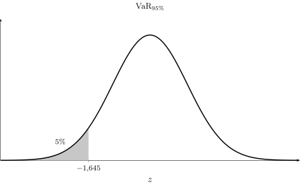
This case study reveals the role of the choice of distribution: if returns followed a heavy-tailed Student’s $t$ rather than a normal, the same confidence level would give a higher VaR — the normal model systematically underestimates the risk of extreme events. The 2008 crisis painfully showed that market tails are heavier than the normal distribution assumes.
Further reading
Polish textbooks
- J. Koronacki, J. Mielniczuk, Statystyka dla studentów kierunków technicznych i przyrodniczych, WNT.
- K. Jajuga (ed.), Zarządzanie ryzykiem, PWN, Warsaw.
World classics
- W. Feller, An Introduction to Probability Theory and Its Applications, Wiley.
- J. Wooldridge, Introductory Econometrics: A Modern Approach, Cengage.
Articles and historical sources
- Student (W. S. Gosset), The Probable Error of a Mean, Biometrika 6 (1908), 1–25. DOI: 10.2307/2331554.
Summary
A probability distribution describes how probable the values of a random variable are — through the density function and the distribution function. The four distributions of inference — the normal, Student’s $t$ (heavier tails when the variance is estimated), chi-square (a sum of squared normal variables), and $F$ (a ratio of normalised chi-square variables) — form a single system growing out of the normal distribution and constitute the apparatus of hypothesis tests. Their generalisation to $\mathbb{R}^n$ links probability theory with the geometry of regression.
Next: The normal distribution
- J. Wooldridge, Introductory Econometrics (Appendix B)
- W. Feller, An Introduction to Probability Theory
- R:
dnorm/pnorm/qnorm,dt/pt/qt,pchisq/qchisq,pf/qf - Python:
scipy.stats.norm,scipy.stats.t,scipy.stats.chi2,scipy.stats.f