The normal distribution

Abstract

The normal (Gaussian) distribution built from the ground up: genesis (de Moivre, Laplace, Gauss, Quetelet), the origin of the bell curve as a limit of the binomial distribution, the density formula and the role of the parameters μ and σ, the 68-95-99.7 rule, standardisation with proof, the z-score, tails and critical values, the bivariate distribution in 3D, elliptical contours, and the multivariate distribution in ℝⁿ. Every concept and every example with its own figure.

The normal distribution — also called Gaussian, or the bell curve — is the most important distribution in statistics and econometrics. Human heights, measurement errors, asset returns: a great many phenomena take the same symmetric shape, densest at the centre and thin at the extremes. This chapter builds it from the ground up: from its genesis and the origin of the bell shape, through the density formula and standardisation, up to the multivariate distribution in the space $\mathbb{R}^n$. Every concept and every example is given its own figure.

The genesis of the normal distribution

The bell curve first appeared in 1733 in the work of Abraham de Moivre as an approximation of the binomial distribution for a large number of trials — a tool for quickly computing probabilities in games of chance. Pierre-Simon Laplace developed this idea into a theory of errors, and in 1809 Carl Friedrich Gauss derived the normal distribution as the law of measurement errors, linking it with the least squares method — hence the name “Gaussian.” In the mid-nineteenth century Adolphe Quetelet showed that human characteristics too (height, chest circumference) follow this curve, making it a symbol of a “law of nature.” We begin by showing where the shape itself comes from.

The origin of the bell shape

The simplest way to see where the bell curve comes from is de Moivre’s observation: the distribution of the number of successes in many coin tosses — the binomial distribution — approximates a smooth bell ever better as the number of trials grows.

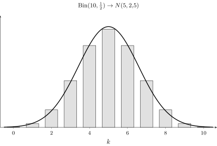
Binomial distribution approximated by a normal curve — The binomial distribution $\mathrm{Bin}(10,\tfrac12)$ (bars) — the number of heads in ten coin tosses — is already close to the normal curve $N(5;2.5)$ (line). The more trials, the more accurate the approximation. This is how de Moivre discovered the bell curve.

This phenomenon has a deep cause — the central limit theorem, according to which the sum of many small, independent influences tends to the normal distribution. This is why the bell appears wherever an outcome is the sum of many factors.

The bell curve of the normal distribution with the 68-95-99.7 rule — The bell curve. The area under the whole curve is $1$ (all cases). Within one standard deviation $\sigma$ of the mean lies $68\%$ of the observations, within two $95\%$, within three $99.7\%$. This is the famous $68$–$95$–$99.7$ rule.

The density formula and the role of the parameters

Definition

Density of the normal distribution

A variable $X$ has a normal distribution $\mathcal{N}(\mu,\sigma^2)$ if its density is

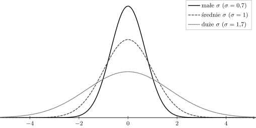
$$ f(x)=\frac{1}{\sigma\sqrt{2\pi}}\,\exp\!\Big(-\frac{(x-\mu)^2}{2\sigma^2}\Big). $$

The parameter $\mu$ is the mean (the location of the peak), and $\sigma$ the standard deviation (the width of the bell). The factor $\tfrac{1}{\sigma\sqrt{2\pi}}$ ensures that the area under the curve is $1$.

The formula reveals the structure of the curve: the kernel $e^{-(x-\mu)^2/(2\sigma^2)}$ is symmetric about $\mu$ and decays the faster the farther from the centre, while the square in the exponent accounts for the rapid decay at the extremes. The parameter $\mu$ shifts the bell along the axis, and $\sigma$ stretches or compresses it.

Three normal curves with different standard deviations — The same family, different parameters. A larger $\sigma$ gives a wider, lower bell (greater spread), a smaller one a narrower, taller bell. Changing $\mu$ would shift the whole bell without changing its shape.

Standardisation and the $z$-score

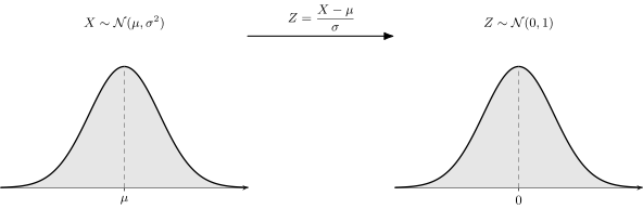
There are infinitely many normal distributions — one for each pair $(\mu,\sigma)$. All of them, however, can be reduced to a single reference, the standard normal distribution $\mathcal{N}(0,1)$, by standardisation:

$$ Z=\frac{X-\mu}{\sigma}. $$

The $z$-score tells how many standard deviations a given value lies above (or below) the mean.

Proof

Standardisation gives mean 0 and deviation 1

Expected value. By linearity $E[aX+b]=aE[X]+b$, and since $Z=\tfrac{1}{\sigma}X-\tfrac{\mu}{\sigma}$: $$E[Z]=\frac{1}{\sigma}E[X]-\frac{\mu}{\sigma}=\frac{\mu}{\sigma}-\frac{\mu}{\sigma}=0.$$
Variance. By the rule $\mathrm{Var}(aX+b)=a^2\mathrm{Var}(X)$ (adding a constant does not change the spread): $$\mathrm{Var}(Z)=\frac{1}{\sigma^2}\mathrm{Var}(X)=\frac{\sigma^2}{\sigma^2}=1.$$
Conclusion. The standard deviation is $\sqrt{1}=1$, so $Z\sim\mathcal{N}(0,1)$ — regardless of the original $\mu$ and $\sigma$. $\;$

∎

Standardisation: from N(mu,sigma) to standard N(0,1) — Standardisation is a shift (subtracting $\mu$ — the centre lands at $0$) and a rescaling (dividing by $\sigma$ — the deviation becomes the unit). The shape of the bell remains unchanged.

The 68-95-99.7 rule in practice

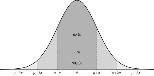
Interpreting the rule.

Suppose adult height has the distribution $\mathcal{N}(\mu=175,\sigma=7)$ cm. Then $68\%$ of people measure $168$–$182$ cm, $95\%$ measure $161$–$189$ cm, and only $0.3\%$ fall outside the range $154$–$196$ cm. The $68$–$95$–$99.7$ rule lets us instantly judge which values are typical and which rare.

Tails and critical values

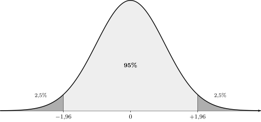
The area under the tail of the $\mathcal{N}(0,1)$ curve is the probability of an outcome “as extreme or more so.” A symmetric cut of $2.5\%$ on each side leaves the central $95\%$ between $-1.96$ and $1.96$ — hence the critical value $1.96$, ubiquitous in statistics.

Tails of the normal distribution beyond plus or minus 1.96 — The area under the tail is a probability. The regions beyond $\pm1.96$ are marked — together $5\%$ ($2.5\%$ on each side). This is the basis of tests at the $5\%$ significance level and of confidence intervals.

A numerical example

An exam score has the distribution $\mathcal{N}(\mu=60,\sigma=10)$. For a person with a score of $75$,

$$ z=\frac{75-60}{10}=1.5, $$

that is, $1.5$ standard deviations above the mean. The area to the left of $z=1.5$ is about $0.933$, so this person scored better than about $93\%$ of the test-takers.

The bivariate and multivariate distribution

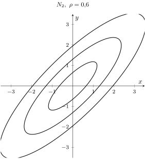
When we study two variables at once (e.g. income and expenditure), the single bell becomes a surface over the plane — the joint density $f(x,y)$. Its peak lies over the mean $(\mu_x,\mu_y)$, and its shape depends on the variances of both variables and their correlation $\rho$: for $\rho\ne 0$ the bell stretches along the diagonal.

Bivariate normal distribution as a 3D surface — The bivariate normal distribution: the joint density $f(x,y)$ is a bell-shaped surface over the plane. With correlation $\rho=0.6$ it is elongated along the diagonal — high values of one variable co-occur with high values of the other.

This surface can be represented in the plane by contours — curves of constant density. For the bivariate distribution these are concentric ellipses, whose orientation reflects the correlation and whose size reflects the distance from the centre measured in standard deviations (the so-called Mahalanobis distance).

Elliptical contours of the bivariate normal distribution — Contours of the bivariate normal distribution ($\rho=0.6$): the curves of constant density are concentric ellipses tilted along the diagonal. The farther from the centre, the lower the density — the ellipses mark regions of equal probability.

The normal distribution in $\mathbb{R}^n$ and the fourth dimension.

For $n$ variables the normal distribution is described by a mean vector $\boldsymbol\mu$ and a covariance matrix $\boldsymbol\Sigma$ (see variance). Its density depends on the expression $(\mathbf{x}-\boldsymbol\mu)^\top\boldsymbol\Sigma^{-1}(\mathbf{x}-\boldsymbol\mu)$ — the squared Mahalanobis distance — whose level sets are hyperellipsoids. In $\mathbb{R}^2$ these are ellipses, in $\mathbb{R}^3$ ellipsoids, and in $\mathbb{R}^4$ and higher solids that cannot be drawn but are studied “layer by layer,” fixing some of the coordinates. The multivariate normal distribution is the foundation of the theory of OLS estimators, which have (approximately) exactly this distribution.

Application — case study: quality control (Six Sigma)

The normal distribution is the foundation of statistical quality control. A machine produces a part with target dimension $\mu$ and natural spread $\sigma$. The customer accepts dimensions within the specification limits $[\mu-3\sigma,\mu+3\sigma]$ (lower and upper, LSL and USL). The $68$–$95$–$99.7$ rule implies that $99.7\%$ of output falls within these limits — leaving $0.3\%$ outside, i.e. $3000$ defects per million (ppm).

The Six Sigma methodology tightens this requirement: the limits are set at $\pm 6\sigma$ from the mean, which (allowing for a typical $1.5\sigma$ process shift) corresponds to just $3.4$ defects per million. The entire methodology is thus a direct application of the tails of the normal distribution.

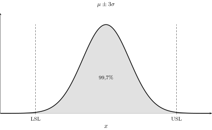
Quality control: specification limits against the normal distribution — Quality control: the product dimension is normally distributed, and the specification limits are set at $\mu\pm3\sigma$. This interval contains $99.7\%$ of output; the area of both tails (beyond the limits) is the defect rate.

This case study shows why the normal distribution is so useful in practice: knowing only $\mu$ and $\sigma$, we can predict the defect rate and design a process to minimise it — without inspecting every single item.