Derivatives — the rate of change

Abstract

The derivative built from the ground up: genesis (Fermat's tangent problem, Newton's fluxions, Leibniz's dx), the difference quotient and the limit, the derivative from the definition step by step, differentiability versus continuity (proof), the rules of differentiation with a derivation of the product rule, the chain rule, derivatives of elementary functions, higher-order derivatives, monotonicity and convexity, Fermat's theorem and Lagrange's mean value theorem, Taylor's formula, economic applications (profit maximisation, elasticity), partial derivatives and the gradient in 3D, and the generalisation to ℝⁿ. Every concept and every example with its own figure.

The derivative measures the rate of change — the instantaneous speed with which the value of a function responds to a change in its argument. In economics it is marginal cost, marginal revenue, and elasticity; in econometrics it is the gradient of the objective function, whose vanishing determines the estimators. This chapter builds the differential calculus from the historical tangent problem, through the difference quotient and the rules of differentiation, up to Taylor’s formula and partial derivatives and the gradient in the space $\mathbb{R}^n$. Every concept and every example is given its own figure, and the key theorems a proof.

The genesis of the concept of a derivative

The derivative grew out of two seemingly distant questions that turned out to be the same problem. The first was the tangent problem: how to draw a line touching a curve at a single point? In the seventeenth century Pierre de Fermat noticed that at an extremum the tangent is horizontal, and he determined it by comparing the values of the function at points separated by an infinitely small quantity. The second was the question of instantaneous velocity: if we know the position of a body as a function of time, how fast is it moving at a given instant — and not merely on average over an interval?

Both questions lead to the same construction. The average velocity over a time interval is the ratio of the distance travelled to the time — geometrically, the slope of a secant of the position graph. The instantaneous velocity arises when the time interval shrinks to zero and the secant becomes a tangent.

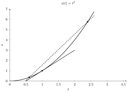
Average velocity (secant) and instantaneous velocity (tangent) on a position graph — Position $s(t)=t^2$ over time. The slope of the secant between two instants is the average velocity on that interval; the slope of the tangent at a single instant is the instantaneous velocity. The derivative is the limit of the former as the time interval shrinks to zero.

Isaac Newton called the instantaneous rate of change a fluxion, and Gottfried Wilhelm Leibniz introduced the notation $\tfrac{dy}{dx}$ as a ratio of infinitely small increments — notation we still use today. A rigorous foundation came only with the limit in Cauchy’s sense, and it is where the definition begins.

Definition of the derivative

Definition

Derivative of a function at a point

The derivative of a function $f$ at a point $x_0$ is the limit of the difference quotient

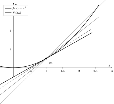
$$ f'(x_0)=\lim_{h\to 0}\frac{f(x_0+h)-f(x_0)}{h}, $$

provided this limit exists and is finite; we then say the function is differentiable at $x_0$. The quotient $\tfrac{f(x_0+h)-f(x_0)}{h}$ is the slope of the secant through the points $\big(x_0,f(x_0)\big)$ and $\big(x_0+h,f(x_0+h)\big)$.

Geometrically the derivative $f'(x_0)$ is the slope of the tangent to the graph at the point $\big(x_0,f(x_0)\big)$: the limiting position of the secants as the second point slides toward the first.

Secants tending to the tangent as h tends to zero — The difference quotient is the slope of the secant through points separated by $h$. As $h\to 0$ the secants (light) rotate to a limiting position — the tangent (dark). Its slope is the value of the derivative.

The derivative from the definition — a full computation

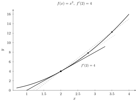
Let us compute the derivative of $f(x)=x^2$ at the point $x_0=2$ directly from the definition. We form the difference quotient:

$$ \frac{f(2+h)-f(2)}{h}=\frac{(2+h)^2-4}{h}=\frac{4+4h+h^2-4}{h}=\frac{4h+h^2}{h}=4+h. $$

As $h\to 0$ the expression $4+h$ tends to $4$. Hence $f'(2)=4$ — the secants with slopes $4+h$ rotate to a tangent of slope $4$. The same computation for an arbitrary $x_0$ would give $f'(x_0)=2x_0$, i.e. the rule $(x^2)'=2x$.

Secants to a parabola converging to a tangent of slope four — The derivative of $f(x)=x^2$ at $x_0=2$ from the definition. The secants joining $(2,4)$ with points $(2+h,(2+h)^2)$ have slopes $4+h$; as $h$ decreases they approach a tangent of slope $4$. Hence $f'(2)=4$.

Tangent to a parabola as the derivative — The derivative $f'(2)=7$ as the slope of the tangent to the graph $f(x)=x^2+3x$ at the point $(2,10)$ — the rate at which the function grows there.

Differentiability versus continuity

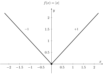
Differentiability is a condition stronger than continuity: every differentiable function is continuous, but not conversely.

Theorem

Differentiability implies continuity

If $f$ has a derivative at $x_0$, then it is continuous at $x_0$. The converse is false: $f(x)=|x|$ is continuous at $0$ but not differentiable.

Proof

Derivative ⇒ continuity

Rewriting the increment. For $h\ne 0$ we write $f(x_0+h)-f(x_0)=\dfrac{f(x_0+h)-f(x_0)}{h}\cdot h$.
Passing to the limit. The first factor tends to the finite number $f'(x_0)$, and the second to $0$, so the product tends to $f'(x_0)\cdot 0=0$.
Conclusion. Hence $f(x_0+h)\to f(x_0)$, i.e. $f$ is continuous at $x_0$. $\;$

∎

Absolute value with a corner at zero — The function $f(x)=|x|$ is continuous everywhere, but at $x=0$ it has a sharp corner: the secants from the left tend to slope $-1$ and from the right to $+1$. The limit of the difference quotient does not exist, so the function is not differentiable at zero.

Rules of differentiation

There is no need to compute the limit each time — operations on functions have their counterparts in operations on derivatives.

Theorem

Basic rules

For differentiable $f,g$ and a constant $c$:

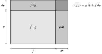
$$ (c)'=0,\qquad (x^n)'=n x^{n-1},\qquad (f+g)'=f'+g',\qquad (c f)'=c f', $$

$$ (fg)'=f'g+fg',\qquad \Big(\frac{f}{g}\Big)'=\frac{f'g-fg'}{g^2},\qquad (g\circ f)'(x)=g'\big(f(x)\big)\,f'(x). $$

Proof

The product rule (Leibniz)

Add-and-subtract trick. In the numerator of the difference quotient of the product we insert an intermediate term: $$\frac{f(x+h)g(x+h)-f(x)g(x)}{h}=\frac{f(x+h)-f(x)}{h}\,g(x+h)+f(x)\,\frac{g(x+h)-g(x)}{h}.$$
Limits of the factors. As $h\to 0$ the first quotient tends to $f'(x)$, the factor $g(x+h)\to g(x)$ (since $g$ is continuous, being differentiable), and the second quotient to $g'(x)$.
Conclusion. Hence $(fg)'(x)=f'(x)g(x)+f(x)g'(x)$. $\;$

∎

Growth of a rectangle's area illustrating the product rule — The product rule geometrically: the area of the rectangle $f\cdot g$ grows by two strips — $g\,df$ and $f\,dg$ — when the sides grow by $df$ and $dg$. The tiny corner $df\,dg$ is negligible in the limit. Hence $d(fg)=g\,df+f\,dg$, i.e. $(fg)'=f'g+fg'$.

The chain rule

The derivative of a composition is the product of the rates of change. If $u=g(x)$ changes at rate $g'(x)$, and $f$ responds to $u$ at rate $f'(u)$, then the composition changes at a rate equal to the product of these rates.

Example

The chain rule in action

For $h(x)=(3x+1)^5$ we take $f(u)=u^5$ and $g(x)=3x+1$. Then $f'(u)=5u^4$ and $g'(x)=3$, so

$$ h'(x)=f'\big(g(x)\big)\,g'(x)=5(3x+1)^4\cdot 3=15(3x+1)^4. $$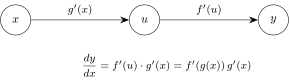

The chain rule as multiplication of rates of change — The chain rule as multiplication of rates: a change in $x$ induces a change in $u=g(x)$ at rate $g'(x)$, which in turn induces a change in $y=f(u)$ at rate $f'(u)$. The total rate $\tfrac{dy}{dx}$ is the product — like the ratio of two gears.

Derivatives of elementary functions

Theorem

Derivatives of the basic functions

$$ (x^n)'=n x^{n-1},\quad (e^x)'=e^x,\quad (a^x)'=a^x\ln a,\quad (\ln x)'=\frac1x,\quad (\sin x)'=\cos x,\quad (\cos x)'=-\sin x. $$

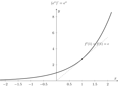
Two of these rules deserve their own figure. The function $e^x$ is its own derivative: at every point the slope of the tangent equals the height of the graph. This distinguishes it among all functions and makes it the foundation of growth models.

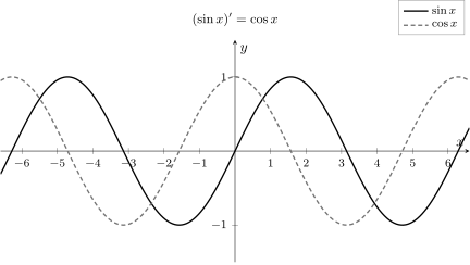
The exponential function whose slope equals its height — The function $e^x$ and its tangent at $x=1$. The slope of the tangent equals the value of the function there, $e\approx 2.718$. The property $(e^x)'=e^x$ holds at every point of the graph.

The derivative of the sine is the cosine: where the sine grows fastest (at zero), the cosine attains its maximum $1$; where the sine reaches a peak, its rate of change — and hence the cosine — is zero.

Sine and cosine as a function and its derivative — The derivative of the sine is the cosine. The cosine reads off the slope of the sine: it is largest where the sine rises most steeply, and vanishes at the peaks and troughs of the sine.

Higher-order derivatives, monotonicity, and convexity

The derivative of the derivative is the second derivative $f''(x)$. The first derivative describes growth, the second describes convexity:

$f'(x)\gt 0$ — increasing function; $f'(x)\lt 0$ — decreasing;
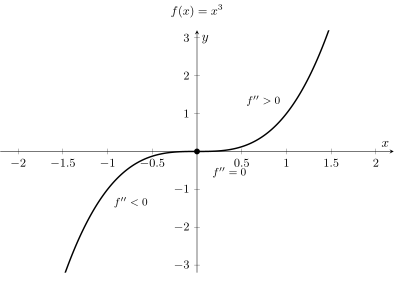
$f''(x)\gt 0$ — convex function (the curve bends upward); $f''(x)\lt 0$ — concave.

A point at which the second derivative changes sign is an inflection point — the boundary between the concave and convex parts.

A cubic function with an inflection point — The function $f(x)=x^3$: for $x\lt 0$ it is concave ($f''=6x\lt 0$), for $x\gt 0$ convex ($f''\gt 0$), and at $x=0$ it has an inflection point where the convexity changes sign.

A function and its derivative — sign of the derivative and monotonicity — The sign of the derivative $f'$ governs the monotonicity of $f$: where $f'\gt 0$, the function increases; where $f'\lt 0$, it decreases. The zeros of $f'$ are critical points — candidates for extrema.

Fermat’s theorem and the classification of extrema

Theorem

Fermat's theorem on extrema

If a differentiable function has a local extremum at an interior point $x_0$, then $f'(x_0)=0$. Points where the derivative vanishes are called stationary or critical.

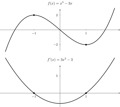
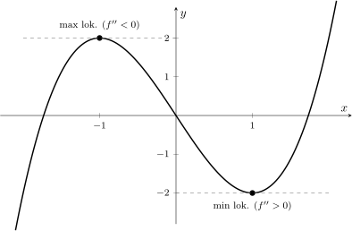
The condition $f'(x_0)=0$ is necessary but not sufficient — the second derivative decides. Let us trace this on a complete example. For $f(x)=x^3-3x$ we have

$$ f'(x)=3x^2-3=3(x-1)(x+1),\qquad f''(x)=6x. $$

The derivative vanishes at $x=\pm 1$. Since $f''(1)=6\gt 0$, there is a local minimum at $x=1$; since $f''(-1)=-6\lt 0$, there is a local maximum at $x=-1$.

Extrema of the function x cubed minus 3x — The function $f(x)=x^3-3x$: at $x=-1$ a local maximum ($f''\lt 0$), at $x=1$ a local minimum ($f''\gt 0$). At both points the tangent is horizontal ($f'=0$). The second derivative decides which stationary point is which extremum.

Lagrange’s mean value theorem

Theorem

Lagrange's mean value theorem

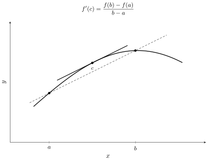
If $f$ is continuous on $[a,b]$ and differentiable on $(a,b)$, then there exists a point $c\in(a,b)$ such that

$$ f'(c)=\frac{f(b)-f(a)}{b-a}. $$

Thus there is a point at which the tangent is parallel to the secant joining the endpoints of the graph.

This theorem links global behaviour (the average change over an interval) with local behaviour (the instantaneous rate) and underlies the proofs of many theorems of analysis. Intuitively: if the average speed on a trip was $90$ km/h, then at some instant the speedometer read exactly $90$.

The mean value theorem — a tangent parallel to the secant — Lagrange’s theorem: for some point $c$ between $a$ and $b$ the tangent to the graph is parallel to the secant joining $\big(a,f(a)\big)$ and $\big(b,f(b)\big)$ — the instantaneous rate equals the average rate.

Taylor’s formula

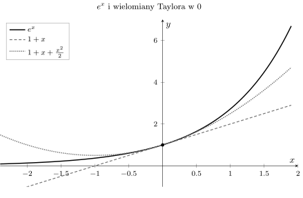
Higher-order derivatives allow a function to be approximated by a polynomial. Taylor’s formula at a point $x_0$ reads

$$ f(x)\approx f(x_0)+f'(x_0)(x-x_0)+\frac{f''(x_0)}{2}(x-x_0)^2+\dots $$

The first term is a constant approximation, the first two give the tangent (a linear approximation), and three give a parabola matched in curvature. The more terms, the better the approximation near $x_0$. In econometrics this is exactly how nonlinear models are linearised around a point.

The exponential function and its Taylor polynomials — The function $e^x$ and its Taylor polynomials at zero: $1+x$ (the tangent) and $1+x+\tfrac{x^2}{2}$ (a parabola). Each successive term improves the fit near zero — first in slope, then in curvature.

Applications in economics and econometrics

Profit maximisation

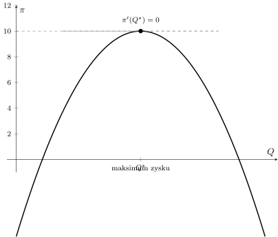
A firm seeks the output $Q$ maximising profit $\pi(Q)$. The necessary condition is the vanishing of the derivative (marginal revenue equals marginal cost), $\pi'(Q^*)=0$, and the sufficient condition for a maximum is a negative second derivative, $\pi''(Q^*)\lt 0$.

Elasticity and log-linear models

The price elasticity of demand, $\varepsilon=\dfrac{dQ}{dP}\cdot\dfrac{P}{Q}$, measures the percentage response of quantity to a percentage change in price. For this reason econometrics often uses the log-linear model

$$ \ln Y=\beta_0+\beta_1\ln X+\varepsilon, $$

in which the coefficient $\beta_1$ is the elasticity, because

$$ \beta_1=\frac{d\ln Y}{d\ln X}=\frac{dY/Y}{dX/X}. $$

The derivative of the logarithm converts absolute changes into relative (percentage) ones — hence the naturalness of this form in modelling.

Partial derivatives and the gradient

In econometrics functions usually depend on several variables — output on capital and labour, the sum of squared residuals on all the parameters $\beta$. The partial derivative $\tfrac{\partial f}{\partial x}$ measures the rate of change when we move only one variable, holding the rest constant.

For $z=f(x,y)$ the partial derivatives $\tfrac{\partial f}{\partial x}$ and $\tfrac{\partial f}{\partial y}$ are the slopes of the surface along the $x$ and $y$ axes. Together they determine the tangent plane to the surface — the two-dimensional counterpart of the tangent line:

$$ z=f(x_0,y_0)+\frac{\partial f}{\partial x}(x-x_0)+\frac{\partial f}{\partial y}(y-y_0). $$

Tangent plane to a paraboloid — partial derivatives — The tangent plane to the surface $z=x^2+y^2$ at the point $(1,1,2)$. Its slopes in the $x$ and $y$ directions are the partial derivatives $\tfrac{\partial f}{\partial x}=2x$ and $\tfrac{\partial f}{\partial y}=2y$, both equal to $2$ at this point. This is the three-dimensional counterpart of the tangent to a curve.

Collected into a vector, the partial derivatives form the gradient $\nabla f=\big(\tfrac{\partial f}{\partial x},\tfrac{\partial f}{\partial y}\big)$. The gradient points in the direction of fastest growth of the function and is perpendicular to the level curves — it is what drives the optimisation algorithms (gradient methods) used in estimation.

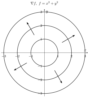
Gradient perpendicular to the level curves — The gradient of $f=x^2+y^2$ is perpendicular to the level curves (circles) and points in the direction of fastest growth — from the centre outward. Gradient-descent algorithms move in the opposite direction, toward the minimum.

The gradient in $\mathbb{R}^n$ and the fourth dimension.

For a function $f\colon\mathbb{R}^n\to\mathbb{R}$ the gradient is a vector of $n$ partial derivatives, $\nabla f=\big(\tfrac{\partial f}{\partial x_1},\dots,\tfrac{\partial f}{\partial x_n}\big)$. The condition for an extremum reads the same as in one variable, except that it concerns all directions at once: $\nabla f=\mathbf{0}$, i.e. the tangent (hyper)plane is horizontal. This is exactly the condition that minimises the sum of squared residuals in the least squares method, where the objective depends on many parameters. The geometry in $\mathbb{R}^4$ and higher cannot be drawn, but the calculus is identical — the gradient and the condition $\nabla f=\mathbf{0}$ work in every dimension, and a four-dimensional surface can be examined “layer by layer,” fixing one coordinate and analysing three-dimensional slices.

Application — case study: a profit-maximising monopolist

Consider a monopolistic firm that, as the sole supplier, sets the price through its level of output. Let the inverse demand function be $P=100-2Q$ and total cost $TC=20Q+200$ (marginal cost $MC=20$, fixed cost $200$). Total revenue is $TR=PQ=100Q-2Q^2$, and profit

$$ \pi(Q)=TR-TC=100Q-2Q^2-(20Q+200)=-2Q^2+80Q-200. $$

The necessary condition for a maximum is the vanishing of the derivative:

$$ \pi'(Q)=-4Q+80=0 \;\Longrightarrow\; Q^\*=20. $$

The second derivative $\pi''(Q)=-4\lt 0$ confirms a maximum. Hence the price $P^\*=100-2\cdot 20=60$ and profit $\pi(20)=600$. Equivalently, $\pi'(Q)=MR-MC$, where marginal revenue $MR=100-4Q$; the condition $\pi'=0$ is the famous rule “marginal revenue = marginal cost” ($100-4Q=20$).

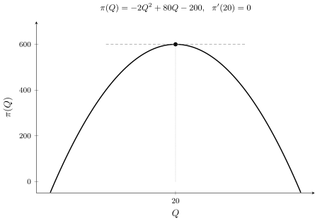
Monopolist profit maximisation — derivative equal to zero — The monopolist’s profit $\pi(Q)=-2Q^2+80Q-200$. The derivative vanishes at $Q^\*=20$ (horizontal tangent), where profit attains its maximum of $600$. This is the computational form of the rule $MR=MC$.

This case study shows the core of mathematical microeconomics: optimal decisions are determined by the first-order condition $\pi'=0$, whose economic content is the equalisation of marginal quantities. The same logic — setting the derivative (gradient) to zero — underlies estimation in econometrics.

Derivatives — the rate of change

The genesis of the concept of a derivative

Definition of the derivative

The derivative from the definition — a full computation

Differentiability versus continuity

Rules of differentiation

The chain rule

Derivatives of elementary functions

Higher-order derivatives, monotonicity, and convexity

Fermat’s theorem and the classification of extrema

Lagrange’s mean value theorem

Taylor’s formula

Applications in economics and econometrics

Profit maximisation

Elasticity and log-linear models

Partial derivatives and the gradient

Application — case study: a profit-maximising monopolist

Further reading

Summary