Correlation and the Pearson coefficient

Abstract

Correlation built from the ground up: genesis (Galton, regression to the mean, Pearson), the definition of the coefficient, the sign of the product of deviations, the picture of r on scatter plots, computation step by step, the geometric interpretation r = cos θ in ℝⁿ, the restriction to linear relationships, Anscombe's quartet, correlation versus causation (the confounder), correlation versus the regression slope, and Spearman's rank correlation. Every concept and every example with its own figure.

Correlation answers the question of whether an increase in one quantity is accompanied by an increase (or decrease) in another — and how strong that relationship is. It is one of the most frequently used and most frequently misused concepts in statistics. This chapter builds the correlation coefficient from the ground up: from its genesis, through the construction of the formula and its geometric meaning in the space $\mathbb{R}^n$, to the interpretive pitfalls — Anscombe’s quartet and the confusion of correlation with causation. Every concept and every example is given its own figure.

The genesis of the concept of correlation

Correlation was born of studies of heredity. In the 1880s Francis Galton, analysing the heights of parents and children, noticed that the children of very tall parents are on average shorter than them — a phenomenon he called regression to the mean. To measure the strength of such a relationship, he introduced a “co-relation coefficient.” This led his pupil Karl Pearson in 1896 to the precise formula for the linear correlation coefficient, used to this day and bearing his name. From the same work grew regression — hence the close kinship of the two concepts, to which we shall return.

Definition of the correlation coefficient

Definition

The Pearson correlation coefficient

The correlation coefficient of variables $x$ and $y$ is

$$ r=\frac{\sum_{i=1}^{n}(x_i-\bar{x})(y_i-\bar{y})}{\sqrt{\sum_{i=1}^{n}(x_i-\bar{x})^2}\,\sqrt{\sum_{i=1}^{n}(y_i-\bar{y})^2}}\in[-1,1]. $$

The numerator is the (scaled) covariance, a measure of how the variables jointly deviate from their means, and the denominator normalises the result to the interval $[-1,1]$, making it dimensionless.

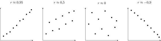
The extreme and middle values have a clear interpretation: $r=+1$ is a perfect increasing relationship (the points lie on a line of positive slope), $r=-1$ a perfect decreasing one, and $r=0$ no linear relationship.

Four scatter plots for different values of correlation — How the correlation coefficient looks on a scatter plot. The closer to $\pm 1$, the more tightly the points line up along a straight line; at $r\approx 0$ the cloud has no clear direction. The sign tells whether the relationship is increasing or decreasing.

Where the sign comes from

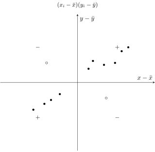
The sign of the product of deviations.

Consider a single observation relative to the centre of the data $(\bar{x},\bar{y})$. When $x_i$ lies above its mean and $y_i$ above its own, the product $(x_i-\bar{x})(y_i-\bar{y})$ is positive; likewise when both are below. When one is above and the other below — the product is negative. The correlation coefficient sums these signals: a preponderance of positive products gives $r\gt 0$, of negative ones $r\lt 0$.

Computation step by step

For the data $x=(1,2,3,4,5)$ and $y=(2,4,5,4,5)$ we have $\bar{x}=3$ and $\bar{y}=4$. The deviations of $x$ are $-2,-1,0,1,2$, and of $y$: $-2,0,1,0,1$. The products of deviations $4,0,0,0,2$ give the numerator $\sum=6$. The sums of squares are $\sum(x_i-\bar{x})^2=10$ and $\sum(y_i-\bar{y})^2=6$. Hence

$$ r=\frac{6}{\sqrt{10}\,\sqrt{6}}=\frac{6}{\sqrt{60}}\approx 0.775. $$

A positive, fairly strong correlation — an increase in $x$ is generally accompanied by an increase in $y$.

Geometric interpretation: $r=\cos\theta$

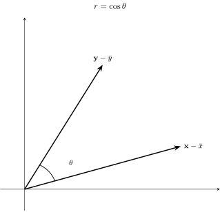
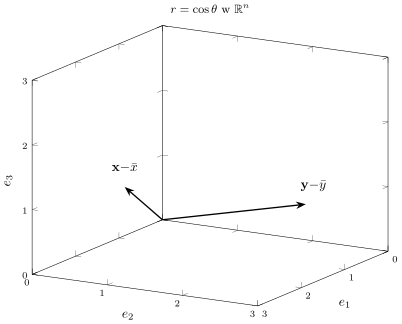
The deepest view of correlation is geometric. Treat the deviations from the means as vectors in the space $\mathbb{R}^n$ (one coordinate per observation): $\mathbf{x}-\bar{x}$ and $\mathbf{y}-\bar{y}$. The numerator of the formula is their dot product, and the denominator is the product of their lengths. By the definition of the dot product it follows that

$$ r=\cos\theta, $$

where $\theta$ is the angle between these vectors. Correlation is the cosine of the angle: aligned vectors ($\theta=0$) give $r=1$, perpendicular ones ($\theta=90°$) give $r=0$, opposite ones ($\theta=180°$) give $r=-1$.

Correlation as the cosine of the angle between deviation vectors — Correlation as the cosine of an angle: the deviation vectors $\mathbf{x}-\bar{x}$ and $\mathbf{y}-\bar{y}$ form an angle $\theta$, and $r=\cos\theta$. A small angle (nearly aligned vectors) means a strong positive correlation.

This interpretation does not depend on the number of observations: the vectors live in $\mathbb{R}^n$, where $n$ is the number of data points. The angle between two vectors is well defined in every dimension, so correlation has the same geometric meaning whether there are three observations or three thousand.

Two deviation vectors in three-dimensional space — The same two deviation vectors in the space $\mathbb{R}^3$ (three observations). The correlation $r=\cos\theta$ is the cosine of the angle between them — a notion meaningful in any dimension $\mathbb{R}^n$, though for many observations it cannot be drawn.

Correlation measures only linear relationships

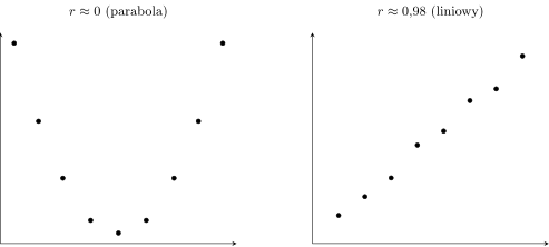
A key limitation: the Pearson coefficient detects only linear relationships. Two variables can be related a hundred percent, yet $r$ will still be zero — if the relationship is curvilinear.

A parabola with zero linear correlation and a linear relationship — On the left a perfect parabola: $y$ is fully determined by $x$, yet $r\approx 0$, because the relationship is not linear (each value of $y$ corresponds to two values of $x$ symmetric about the vertex). On the right a linear relationship gives $r\approx 0.98$. Always visualise the data before trusting a single number.

Anscombe’s quartet

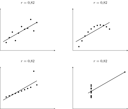
This is shown most strikingly by Anscombe’s quartet (1973): four data sets with identical statistics — the same mean, variance, correlation $r=0.82$, and the same regression line — yet completely different shapes. Only the plot reveals that the first is linear, the second curvilinear, the third distorted by a single outlier, and the fourth resting on one observation.

Correlation versus causation

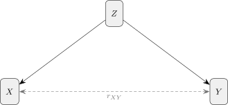
This is perhaps the most important sentence in all of applied statistics. Correlation does not prove causation. Two quantities can rise together though neither influences the other — because both depend on a common, hidden third variable (a so-called confounder).

Confounder diagram: a common cause of two correlated variables — The classic example: ice cream sales ($X$) and the number of drownings ($Y$) rise together, giving a high $r$. But ice cream does not drown people — both quantities are driven by heat ($Z$). The correlation between $X$ and $Y$ is spurious, induced by the common cause $Z$.

This is the origin of all causal econometrics — methods such as instrumental variables, difference-in-differences, and experiments, which let us go beyond mere correlation and make claims about cause.

Correlation versus the regression slope

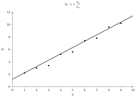
Correlation and the regression slope are kindred but not identical concepts. They are linked by the formula

$$ b_1=r\,\frac{s_y}{s_x}. $$

Both have the same sign, but a different nature: $r$ is dimensionless and always lies in $[-1,1]$, while the slope $b_1$ has units (e.g. “dollars per year of experience”). Correlation measures the strength of the linear relationship, the slope its steepness.

A cloud of points with a regression line — correlation versus slope — A cloud of points with a fitted regression line. The correlation $r$ tells how tightly the points cluster around the line, and the slope $b_1=r\,s_y/s_x$ tells how steep the line itself is. Two different quantities of the same sign.

Spearman’s rank correlation

When the relationship is monotonic but nonlinear (e.g. exponential), the Pearson coefficient underestimates it. In such cases one uses Spearman’s rank correlation — the Pearson coefficient computed not on the values but on their ranks (positions in the ordering). It measures whether both variables rise together, regardless of whether the rise is linear.

Application — case study: portfolio diversification

Correlation is the heart of diversification — the principle “don’t put all your eggs in one basket.” Consider an equally weighted portfolio of two assets, each with standard deviation $\sigma=20\%$. The portfolio risk depends on the correlation $\rho$ of their returns:

$$ \sigma_p=\sqrt{\tfrac14\sigma^2+\tfrac14\sigma^2+2\cdot\tfrac12\cdot\tfrac12\rho\sigma^2}=\sigma\sqrt{\tfrac{1+\rho}{2}}=0.2\sqrt{\tfrac{1+\rho}{2}}. $$

The result is striking: when the assets are perfectly correlated ($\rho=1$), portfolio risk is still $20\%$ — diversification achieves nothing. But at $\rho=0$ it falls to $0.2/\sqrt2\approx 14.1\%$, and at $\rho=-1$ to zero: oppositely correlated assets cancel each other’s fluctuations. The lower the correlation, the greater the benefit of combining assets.

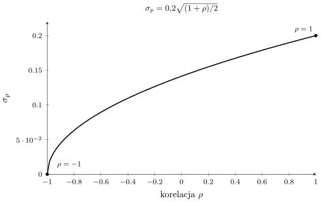
Portfolio risk decreasing as asset correlation falls — Portfolio risk $\sigma_p$ as a function of the correlation $\rho$ of two assets (equal weights, $\sigma=20\%$). Lower correlation reduces risk: at $\rho=1$ there is no benefit, at $\rho=-1$ risk vanishes. This is the mathematical essence of diversification.

This case study explains why investors seek assets with low or negative correlation, and why the correlation coefficient — though it measures “only” a linear relationship — is one of the most important numbers in finance. It also recalls this chapter’s warning: correlations can be unstable and, in a crisis, may rise sharply, weakening diversification.