Limits and continuity
Limits built from the ground up: genesis (Zeno's paradoxes, the infinitesimals of Newton and Leibniz, the rigour of Cauchy and Weierstrass), the limit of a sequence with the ε–N definition, the limit of a function with the ε–δ definition, Heine's definition, the laws of limits with justification, one-sided limits, indeterminate forms, the squeeze theorem with proof, the limit of sin x / x, limits at infinity and the number e, continuity and its types, the intermediate value theorem, limits of functions of several variables in 3D, and the generalisation of continuity to ℝⁿ. Every concept and every example with its own figure.
The limit is the foundation of all of differential and integral calculus. It answers a single question: what value does a function approach as its argument approaches a given point? Without this concept one can define neither the derivative — the instantaneous rate of change — nor the integral — a sum of infinitely many infinitely small terms. This chapter builds the notion of the limit from its historical sources, through rigorous definitions, up to limits and continuity of functions of several variables. Every concept and every example is given its own figure, and the key theorems a proof.
The genesis of the concept of a limit
The idea of the limit grew out of attempts to tame infinity. As early as antiquity, Zeno of Elea formulated paradoxes of motion that we now understand as the problem of summing infinitely many ever-smaller quantities. In the dichotomy paradox, to traverse a segment one must first cover its half, then half of the remainder, then half of the next remainder, and so on without end. Zeno concluded that motion is impossible, since infinitely many acts must be performed. The modern answer is: the infinite sum $\tfrac12+\tfrac14+\tfrac18+\dots$ has a finite limiting value equal to $1$.

In the seventeenth century Isaac Newton and Gottfried Wilhelm Leibniz built the differential calculus using infinitely small quantities — entities smaller than every positive number yet different from zero. The calculus worked superbly, but its foundations were obscure, as the philosopher George Berkeley aptly pointed out, calling the infinitesimals “ghosts of departed quantities.” Only in the nineteenth century did Augustin-Louis Cauchy, and then Karl Weierstrass, replace the hazy infinitesimals with a rigorous definition of the limit based on inequalities — the famous $\varepsilon$–$\delta$ language. It underlies today’s analysis, and it is where the systematic exposition begins.
The limit of a sequence
The simplest limit passage is the limit of a sequence — a function defined on the natural numbers, $a_1,a_2,a_3,\dots$. We ask whether the terms cluster around a certain number as the index $n$ grows without bound.
Consider the sequence $a_n=\tfrac{1}{n}$. The successive terms are $1,\tfrac12,\tfrac13,\tfrac14,\dots$ — they decrease and approach zero, though they never reach it. We say the sequence is convergent to the limit $0$.
A number $L$ is the limit of a sequence $(a_n)$, written $\lim_{n\to\infty}a_n=L$, if for every number $\varepsilon\gt 0$ there exists an index $N$ such that for all $n\gt N$
$$ |a_n-L|\lt\varepsilon. $$In words: however narrow a band $(L-\varepsilon,\,L+\varepsilon)$ around the limit we choose, from some point on all terms of the sequence stay within it.
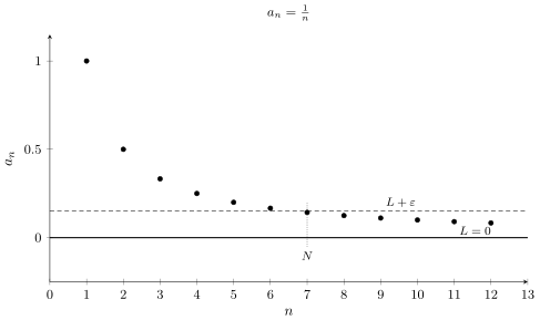
For $a_n=\tfrac1n$ and a given $\varepsilon$ it suffices to take $N=\lceil 1/\varepsilon\rceil$: then for $n\gt N$ we have $\tfrac1n\lt\tfrac1N\le\varepsilon$. The check of the inequality $|a_n-0|\lt\varepsilon$ is thus complete — the definition is satisfied and the limit is $0$.
The limit of a function
Let us turn to functions of a real variable. Consider
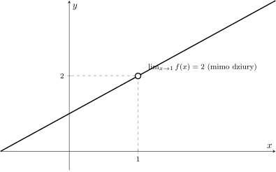
$$ f(x)=\frac{x^2-1}{x-1}. $$At the point $x=1$ the function is undefined (the denominator vanishes). Let us nevertheless study its behaviour near one, substituting arguments ever closer to $1$:
| $x$ | $0.9$ | $0.99$ | $0.999$ | $\to 1 \leftarrow$ | $1.001$ | $1.01$ | $1.1$ |
|---|---|---|---|---|---|---|---|
| $f(x)$ | $1.9$ | $1.99$ | $1.999$ | ? | $2.001$ | $2.01$ | $2.1$ |
The values cluster around $2$ from both sides. This is explained by an algebraic transformation: for $x\ne 1$
$$ \frac{x^2-1}{x-1}=\frac{(x-1)(x+1)}{x-1}=x+1\;\xrightarrow{x\to1}\;2. $$The limit “sees” the value toward which the graph heads, regardless of the fact that the function does not exist at the point itself. We write $\lim_{x\to1}f(x)=2$.
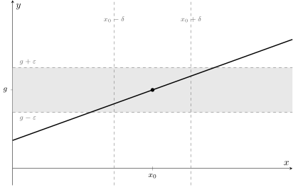
A number $g$ is the limit of a function $f$ at a point $x_0$, written $\lim_{x\to x_0}f(x)=g$, if for every $\varepsilon\gt 0$ there exists $\delta\gt 0$ such that
$$ 0\lt|x-x_0|\lt\delta \;\Longrightarrow\; |f(x)-g|\lt\varepsilon. $$In words: however narrow a band $[g-\varepsilon,\,g+\varepsilon]$ around the limit we choose, there exists a neighbourhood of $x_0$ in which the whole graph lies within that band. The condition $0\lt|x-x_0|$ excludes the point $x_0$ itself — the limit does not depend on the value there.
Heine’s (sequential) definition and its equivalence.
There is a second, equivalent definition of the limit, formulated by Heinrich Heine: $\lim_{x\to x_0}f(x)=g$ if and only if for every sequence of arguments $x_n\to x_0$ (with $x_n\ne x_0$) the sequence of values satisfies $f(x_n)\to g$. This definition is convenient for showing that a limit does not exist: it suffices to exhibit two sequences of arguments tending to $x_0$ for which the values tend to different numbers.
The laws of limits
Limits respect the arithmetic operations, which allows them to be computed without returning to the definition each time.
If the limits $\lim f(x)$ and $\lim g(x)$ (at the same point) exist and are finite, then
$$ \lim(f+g)=\lim f+\lim g,\qquad \lim(f\cdot g)=\lim f\cdot\lim g, $$$$ \lim\frac{f}{g}=\frac{\lim f}{\lim g}\;(\text{when }\lim g\ne 0),\qquad \lim(c\cdot f)=c\cdot\lim f. $$These formulas follow directly from the $\varepsilon$–$\delta$ definition. For the sum, if $f$ stays within distance $\tfrac{\varepsilon}{2}$ of its limit and $g$ within $\tfrac{\varepsilon}{2}$ of its own, then by the triangle inequality $f+g$ stays within distance $\varepsilon$ of the sum of the limits. Analogous, if somewhat longer, computations give the remaining formulas.
Indeterminate forms
Direct substitution sometimes leads to undefined expressions: $\tfrac{0}{0}$, $\tfrac{\infty}{\infty}$, $\infty-\infty$, $0\cdot\infty$. These have no predetermined value — the result depends on the particular functions and requires a transformation (simplification, substitution, or l’Hospital’s rule, which we introduce with derivatives). The example $\tfrac{x^2-1}{x-1}$ above was precisely a $\tfrac{0}{0}$ form resolved by cancellation.
The squeeze theorem
One of the most effective tools for finding limits is to trap a function between two others with a known common limit.
If in some neighbourhood of the point $x_0$ (apart from $x_0$ itself) we have
$$ g(x)\le f(x)\le h(x), $$and $\lim_{x\to x_0}g(x)=\lim_{x\to x_0}h(x)=L$, then also $\lim_{x\to x_0}f(x)=L$.
- Fixing the band. Let $\varepsilon\gt 0$. By assumption there exist $\delta_1,\delta_2$ such that for $0\lt|x-x_0|\lt\delta_1$ we have $|g(x)-L|\lt\varepsilon$, and for $0\lt|x-x_0|\lt\delta_2$ we have $|h(x)-L|\lt\varepsilon$.
- Common neighbourhood. Taking $\delta=\min(\delta_1,\delta_2)$, for $0\lt|x-x_0|\lt\delta$ we have simultaneously $L-\varepsilon\lt g(x)$ and $h(x)\lt L+\varepsilon$.
- Conclusion from the inequalities. Since $g(x)\le f(x)\le h(x)$, we obtain $L-\varepsilon\lt f(x)\lt L+\varepsilon$, i.e. $|f(x)-L|\lt\varepsilon$. By the arbitrariness of $\varepsilon$, $\lim_{x\to x_0}f(x)=L$. $\;$
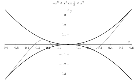
The limit $\dfrac{\sin x}{x}$
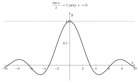
A classic application of the squeeze theorem is the fundamental limit
$$ \lim_{x\to0}\frac{\sin x}{x}=1. $$Comparing the areas of a circular sector and two triangles yields, for small $x\gt 0$, the inequalities $\cos x\le\tfrac{\sin x}{x}\le 1$. Since $\cos x\to 1$ as $x\to0$, the middle function is trapped between two quantities tending to $1$ — hence the limit equals $1$. The expression is a $\tfrac{0}{0}$ form, and its value $1$ underlies the derivative of the sine.
Limits at infinity
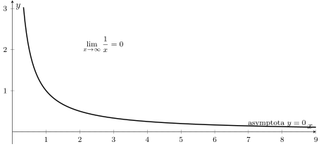
Limits at infinity describe the long-run behaviour of a function — what happens to the values as the argument grows without bound.
The simplest example is $\lim_{x\to\infty}\tfrac1x=0$: the values decrease ever more slowly, approaching the horizontal axis but never reaching it. The line $y=0$ is called a horizontal asymptote.
For a rational function the limit at infinity is determined by the ratio of the highest-degree terms. For $f(x)=\tfrac{2x^2+1}{x^2+3}$ we divide numerator and denominator by $x^2$:
$$ \frac{2x^2+1}{x^2+3}=\frac{2+\tfrac{1}{x^2}}{1+\tfrac{3}{x^2}}\;\xrightarrow{x\to\infty}\;\frac{2+0}{1+0}=2. $$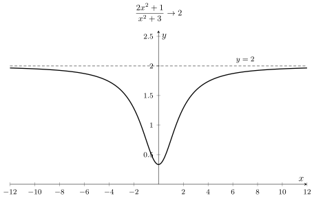
The number $e$ and continuous compounding
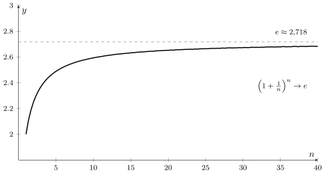
Especially important is the limit defining Euler’s number:
$$ \lim_{n\to\infty}\left(1+\frac{1}{n}\right)^n=e\approx 2.718. $$The expression has the indeterminate form $1^\infty$: the base tends to $1$ while the exponent grows without bound, and the two tendencies balance, giving a finite limit.
Capital $K_0$ at an annual rate $r$, compounded $n$ times a year, after one year equals $K_0\big(1+\tfrac{r}{n}\big)^n$. Under continuous compounding ($n\to\infty$) the substitution $m=\tfrac{n}{r}$ gives
$$ \lim_{n\to\infty}K_0\Big(1+\frac{r}{n}\Big)^n=K_0\lim_{m\to\infty}\Big(1+\frac{1}{m}\Big)^{mr}=K_0\,e^{r}. $$The number $e$ thus arises naturally in finance as the limit of unbounded densification of compounding.
One-sided limits
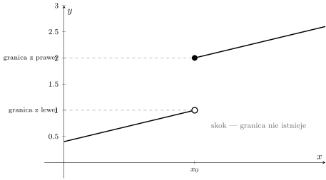
Sometimes a function approaches different values as the argument tends to $x_0$ from the left and from the right. We then define the one-sided limits $\lim_{x\to x_0^-}f(x)$ and $\lim_{x\to x_0^+}f(x)$.
The (two-sided) limit exists if and only if both one-sided limits exist and are equal:
$$ \lim_{x\to x_0}f(x)=g \iff \lim_{x\to x_0^-}f(x)=\lim_{x\to x_0^+}f(x)=g. $$A typical example of divergent one-sided limits is a step function — a model of a tax threshold or a threshold fee. At the point of the jump the limit from the left is lower than the limit from the right, so the two-sided limit does not exist.
Continuity of a function
Continuity is the property of a function whose graph can be drawn “without lifting the pencil.” Formally it reduces to agreement of the value with the limit.
A function $f$ is continuous at a point $x_0$ if three conditions hold:
$$ \text{(1) }f(x_0)\text{ is defined},\qquad \text{(2) }\lim_{x\to x_0}f(x)\text{ exists},\qquad \text{(3) }\lim_{x\to x_0}f(x)=f(x_0). $$A function continuous at every point of a set is called continuous on that set.
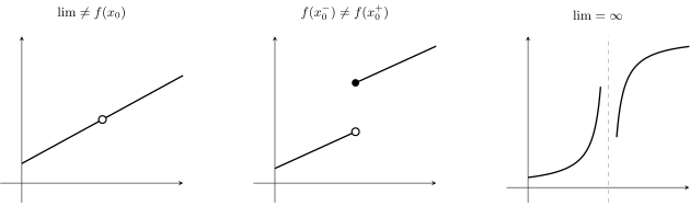
Types of discontinuity
Violating any of the three conditions gives a discontinuity. We distinguish three basic types:
- removable — the limit exists, but the value at the point is different or undefined (a “hole” in the graph);
- jump — the one-sided limits exist but differ (a jump in value; e.g. tax thresholds);
- infinite — the function tends to $\pm\infty$, a vertical asymptote appears (e.g. cost growing to infinity at a capacity constraint).
The intermediate value theorem
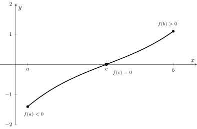
Continuity has profound consequences. The most important is the guarantee that a continuous function cannot “skip” any intermediate value.
In economics this theorem guarantees the existence of an equilibrium price: if excess demand is positive at a low price and negative at a high price, and varies continuously, then there exists a price at which excess demand is zero — the market clears.
Limits and continuity of functions of several variables
For a function of one variable the limit exists when both sides — from the left and from the right — give the same value; there are only two possible paths of approach. For a function $z=f(x,y)$ the situation is substantially richer: the point $(0,0)$ can be approached along infinitely many paths — along the axes, along any straight line, along a parabola — and the limit exists only if every path leads to the same value.
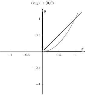
This is shown by the classic counterexample $z=\dfrac{xy}{x^2+y^2}$. Along the axes ($x=0$ or $y=0$) the function takes the value $0$, but along the line $y=x$ we obtain $\tfrac{x\cdot x}{x^2+x^2}=\tfrac12$. Two paths give two different values, so the limit at $(0,0)$ does not exist, even though the function is smooth apart from that single point.

By contrast, the function $z=e^{-(x^2+y^2)}$ is continuous everywhere: its surface has no holes or jumps, and the value at every point agrees with the limit regardless of the path of approach.

Continuity in the space $\mathbb{R}^n$ and the fourth dimension.
The $\varepsilon$–$\delta$ definition carries over to any dimension unchanged: the limit $\lim_{\mathbf{x}\to\mathbf{x}_0}f(\mathbf{x})=g$ means that for every $\varepsilon\gt 0$ there exists $\delta\gt 0$ such that $f(\mathbf{x})$ lies within distance less than $\varepsilon$ of $g$ whenever the distance between the points $\mathbf{x}$ and $\mathbf{x}_0$ in $\mathbb{R}^n$ is less than $\delta$. Only the number of paths of approach grows: in $\mathbb{R}^2$ we approach a point from infinitely many directions, in $\mathbb{R}^3$ from a whole ball of directions, in $\mathbb{R}^4$ and higher from a solid of directions that cannot be drawn. A four-dimensional limit can be viewed “layer by layer,” fixing the fourth coordinate and examining the continuity of each three-dimensional slice. The function is continuous when all these paths and all these layers agree with one another.
Significance for economics and econometrics
- Limits define the derivative — marginal cost and revenue — and the integral as a sum of infinitely many terms.
- Continuity of demand and supply functions guarantees (through the intermediate value theorem) the existence of an equilibrium price.
- Limits at infinity describe long-run analysis and the present value of a perpetuity.
- Discontinuities model tax thresholds, price jumps, and “yes/no” decisions.
Application — case study: continuous compounding
Limits have a direct application in finance. A bank offers a deposit at a nominal annual rate $r$, compounded $n$ times a year. After one year, capital of $1$ grows to $\big(1+\tfrac{r}{n}\big)^n$. The question is: what happens as compounding becomes ever more frequent — monthly, daily, every second?
The answer is a limit. Taking $r=1$ (a rate of $100\%$) for simplicity, we observe the sequence
$$ n=1:\;2.00,\quad n=2:\;2.25,\quad n=4:\;2.44,\quad n=12:\;2.61,\quad \dots\;\longrightarrow\; e\approx 2.718. $$The value does not grow without bound — it converges to Euler’s number. For an arbitrary rate $r$, the analogous limit gives continuous compounding: $\lim_{n\to\infty}\big(1+\tfrac{r}{n}\big)^n=e^r$. Capital $K_0$ after time $t$ is therefore $K_0 e^{rt}$ — the formula underlying the valuation of financial instruments and growth models.
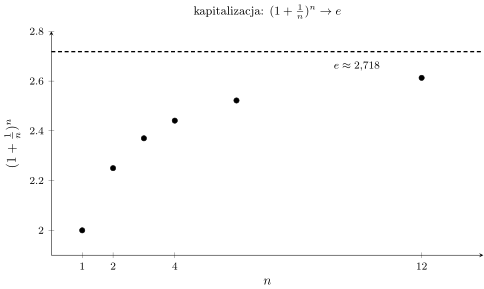
This case study shows that the limit is no abstraction: the difference between monthly and continuous compounding is a concrete sum of money, and computing it requires precisely a limit passage.
Further reading
Polish textbooks
- G. M. Fichtenholz, Differential and Integral Calculus, vol. I, PWN.
- K. Kuratowski, Differential and Integral Calculus, PWN.
World classics
- W. Rudin, Principles of Mathematical Analysis, McGraw-Hill, 1976.
- T. M. Apostol, Mathematical Analysis, Addison-Wesley, 1974.
Articles and historical sources
- J. V. Grabiner, Who gave you the epsilon? Cauchy and the origins of rigorous calculus, The American Mathematical Monthly 90 (1983), 185–194. DOI: 10.2307/2975545.
Summary
The limit formalises the intuition of “approaching” — from Zeno’s paradoxes, through the infinitesimals of Newton and Leibniz, to the rigorous $\varepsilon$–$\delta$ language of Cauchy and Weierstrass. The limit of a sequence, the limit of a function, the laws of limits, the squeeze theorem, and the notion of continuity form the foundation on which derivatives, integrals, and the entire analysis of functions of several variables in $\mathbb{R}^n$ rest.
- G. M. Fichtenholz, Differential and Integral Calculus, vol. I
- W. Rudin, Principles of Mathematical Analysis
- Python:
sympy.limit(f, x, x0)— symbolic limit;sympy.limit(f, x, oo) - R: numerical check of a limit by refining the arguments