Functions and their properties

Abstract

Functions built from the ground up: the genesis of the concept (Oresme, Euler, Dirichlet), from relation to function, the vertical line test, domain and codomain, a full catalogue of elementary functions with derivations, properties (monotonicity, extrema, parity, periodicity, convexity, asymptotes), graph transformations, composition, the inverse function, injection/surjection/bijection, functions of several variables in 3D, and the idea of the fourth dimension with the generalisation to $\mathbb{R}^n$. Every concept and every example with its own figure.

The function is one of the most important concepts in all of mathematics and, at the same time, the foundation of econometrics, in which a model is a function linking explanatory variables to the explained variable. This chapter begins with the genesis of the concept, then builds it from the ground up — from a general relation to a function in the strict sense — and leads the reader through a complete catalogue of elementary functions, their properties, transformations, and the generalisation to functions of several variables and the space $\mathbb{R}^n$. We apply one rule consistently: every concept and every example is given its own figure.

The genesis of the concept of a function

The notion of a function did not appear ready-made; it took shape over several centuries together with a growing understanding of the dependence between varying quantities.

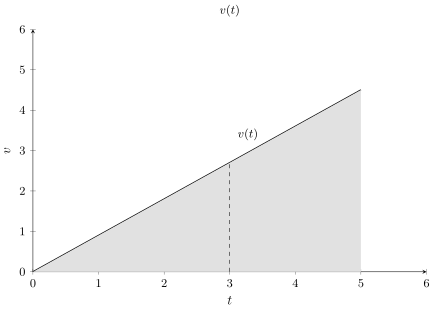
The first significant step was the fourteenth-century work of Nicole Oresme, who represented a quantity varying in time (for example, velocity) as the height of a segment raised above a time axis. This was the germ of the graph: a dependence of one quantity on another becomes a geometric figure, and the area beneath it becomes an accumulated quantity (distance). This is the direct ancestor of today’s function graph and of the definite integral.

An early idea of the graph: velocity as a height above the time axis — Oresme’s idea (the “latitude of forms”): a velocity $v(t)$ varying in time is represented as a height above the time axis. The area of the region under the graph corresponds to the distance travelled. This is the historical beginning of graphing the dependence of one quantity on another.

The term functio was introduced by Gottfried Wilhelm Leibniz around the turn of the eighteenth century, initially for quantities associated with a curve. The modern notation $y=f(x)$ is due to Leonhard Euler (18th century), who understood a function as an analytic expression — a formula. Only in the nineteenth century did Peter Gustav Lejeune Dirichlet free the concept from the need to possess a formula: a function is any single-valued assignment, regardless of whether we can write it as a simple expression. This general definition holds to this day, and it is where the systematic exposition begins.

From relation to function

To define a function rigorously, we begin with a more general notion — the relation. Given two sets $X$ and $Y$, any set of ordered pairs $(x,y)$, where $x\in X$ and $y\in Y$, is called a relation between $X$ and $Y$. A relation links elements of the two sets but imposes no restriction: a single element $x$ may be paired with many elements $y$ or with none.

A function is a special case of a relation — one in which the assignment is single-valued and everywhere defined.

Definition

Function

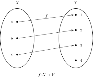
A function from a set $X$ to a set $Y$ is a rule $f$ that assigns to every element $x\in X$ exactly one element $y\in Y$. We write

$$ f\colon X \to Y, \qquad y = f(x), $$

where $x$ is the argument (independent variable), $y$ is the value (dependent variable), and $f$ is the assignment rule. The set $X$ is called the domain and $Y$ the codomain.

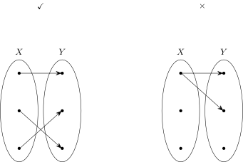
The two conditions in the definition are equally important. The word “every” means that the rule must be defined for all arguments of the domain. The words “exactly one” rule out a situation in which a single argument corresponds to two different values. It is precisely this second condition that distinguishes a function from an arbitrary relation.

Mapping diagram: each argument is assigned exactly one value — A function assigns to every element of the domain $X$ exactly one element of the codomain $Y$. From each argument there issues exactly one arrow.

Comparison: a function versus a many-valued assignment — On the left — an assignment that is a function (one arrow from each $x$). On the right — an assignment that is not a function: a single argument corresponds to two different values, so the single-valuedness condition is violated.

The graph of a function and the vertical line test

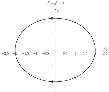
The graph of a function $f$ is the set of all pairs $(x,f(x))$ represented as points of the plane. The single-valuedness condition has a clear geometric reading: if a given $x$ corresponded to two values, they would lie one above the other — on the same vertical line. Hence a simple test.

The vertical line test.

A curve in the plane is the graph of some function if and only if every vertical line meets it at most once. Two intersections would mean two values for a single argument.

Vertical line test: a circle intersected twice — The circle $x^2+y^2=4$ is not the graph of a function: the vertical line $x=1$ meets it in two points, so a single argument would correspond to two values.

Evaluating a function

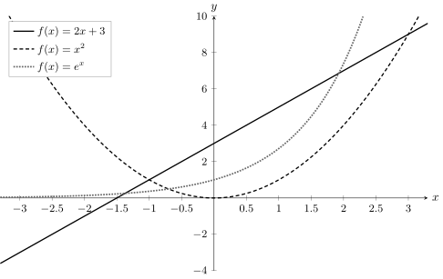
Evaluating a function consists in substituting a number for the argument. Consider $f(x)=2x+3$. Then

$$ f(0)=2\cdot 0+3=3,\qquad f(1)=2\cdot 1+3=5,\qquad f(-2)=2\cdot(-2)+3=-1. $$

The graph lets us read these values off: the argument is chosen on the horizontal axis, and the value is read on the vertical axis above it.

Graphs of a linear, a quadratic, and an exponential function — Three basic functions: the linear $2x+3$ grows with constant slope, the quadratic $x^2$ forms a parabola, and the exponential $e^x$ grows ever faster. From each, the value at a point is read as the height of the graph above the argument.

Domain and codomain

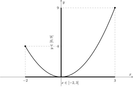
In practice the domain is usually not an abstract set $X$, but the set of all arguments for which the formula makes sense — the natural domain.

Domain ($D_f$) — the set of permitted arguments $x$.
Range ($ZW_f$) — the set of all values $y$ actually attained.

Three rules account for most domain restrictions:

$f(x)=\dfrac{1}{x}$ requires $x\ne 0$ (we do not divide by zero);
$f(x)=\sqrt{x}$ requires $x\ge 0$ (we do not take square roots of negative numbers over the reals);
$f(x)=\ln x$ requires $x\gt 0$ (the logarithm exists only for positive arguments).

Consider an example combining two conditions: $f(x)=\dfrac{\sqrt{x-1}}{x-3}$. The root requires $x-1\ge 0$, i.e. $x\ge 1$; the denominator requires $x\ne 3$. Hence $D_f=[1,3)\cup(3,\infty)$.

Domain and range of a quadratic function — For the function $f(x)=x^2$ restricted to the domain $[-2,3]$, the range is $[0,9]$. The dashed lines show how the endpoints of the domain map to the endpoints of the range.

A catalogue of elementary functions

Elementary functions are the building blocks from which models are made. Below we treat them in turn, deriving the key properties and illustrating each with its own figure.

The linear function

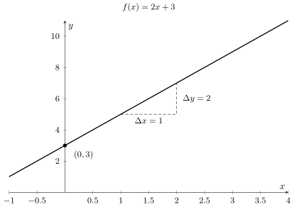
A linear function has the form $f(x)=ax+b$. The coefficient $a$ is the slope: when the argument increases by $1$, the value changes by $a$. The number $b$ is the intercept — the value at $x=0$, that is, the ordinate where the graph crosses the vertical axis.

Let us derive the meaning of the slope. For two arguments $x_1\ne x_2$,

$$ \frac{f(x_2)-f(x_1)}{x_2-x_1}=\frac{(ax_2+b)-(ax_1+b)}{x_2-x_1}=\frac{a(x_2-x_1)}{x_2-x_1}=a. $$

The ratio of the increment of the value to the increment of the argument is constant and equal to $a$ — the defining feature of a linear function and the germ of the notion of the derivative.

A linear function with a slope triangle — The function $f(x)=2x+3$. The intercept $3$ is the point where the graph crosses the vertical axis. The slope triangle shows that an argument increment $\Delta x=1$ corresponds to a value increment $\Delta y=2$, so the slope is $2$.

Polynomials

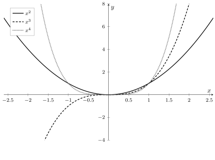
A polynomial is a sum of powers of the argument: $f(x)=a_n x^n+\dots+a_1 x+a_0$. The number $n$ (the highest power with a nonzero coefficient) is called the degree. The higher the degree, the more bends the graph may have. Even powers ($x^2,x^4$) give graphs symmetric about the vertical axis; odd ones ($x^3$) are symmetric about the origin.

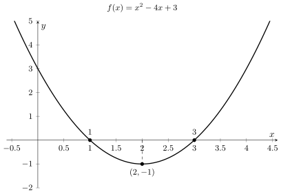
Consider the quadratic polynomial $f(x)=x^2-4x+3$. We find the roots by solving $x^2-4x+3=0$; factoring as $(x-1)(x-3)=0$ gives $x=1$ and $x=3$. The vertex of the parabola has abscissa $x_v=-\tfrac{b}{2a}=\tfrac{4}{2}=2$, and the value there is $f(2)=4-8+3=-1$. This is the complete information about the shape.

A parabola with marked roots and vertex — The polynomial $f(x)=x^2-4x+3$. The roots $x=1$ and $x=3$ are the points where it crosses the horizontal axis, and the vertex $(2,-1)$ is the lowest point of the parabola — all obtained by calculation.

Polynomials: x squared, cubic, and fourth degree — The higher the degree of the polynomial, the steeper the growth at the extremes. The even powers $x^2$ and $x^4$ open upward and are symmetric about the vertical axis, while $x^3$ passes through the origin symmetrically about it.

The rational function

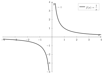
A rational function is a quotient of two polynomials. The simplest example is the hyperbola $f(x)=\dfrac{1}{x}$. At $x=0$ the function is undefined, and near that point the values grow without bound in magnitude — the line $x=0$ is called a vertical asymptote. As $x$ grows without bound, the values tend to zero — the horizontal axis is a horizontal asymptote.

Root and absolute value

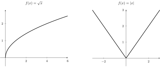
The function $f(x)=\sqrt{x}$ is defined only for $x\ge 0$ and grows ever more slowly — it is the inverse of $x^2$ restricted to nonnegative arguments. The function $f(x)=|x|$ takes the value $x$ for $x\ge 0$ and $-x$ for $x\lt 0$, giving the characteristic “V” shape with its vertex at zero.

The square root function and the absolute value — The root $\sqrt{x}$ exists only for $x\ge 0$ and grows ever more slowly. The absolute value $|x|$ forms a symmetric “V” with its vertex at the origin.

Exponential and logarithmic functions

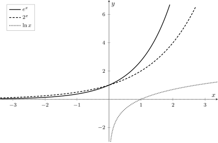
The exponential function $f(x)=a^x$ (for a base $a\gt 0$, $a\ne 1$) grows faster the larger the base, and never takes negative values. A special role is played by the base $e\approx 2.718$, for which the growth rate at every point equals the value of the function.

We define the logarithm as the function inverse to the exponential: $\log_a y$ is the exponent to which $a$ must be raised to obtain $y$. Hence the equivalence

$$ y=a^x \quad\Longleftrightarrow\quad x=\log_a y. $$

The natural logarithm $\ln x=\log_e x$ exists only for $x\gt 0$ and grows very slowly. Both functions are a pillar of growth models and of the normal distribution.

Exponential functions and the logarithm — The functions $e^x$ and $2^x$ grow exponentially and remain positive. The logarithm $\ln x$ — the function inverse to $e^x$ — grows slowly and is defined only for $x\gt 0$.

Trigonometric functions

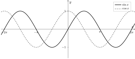
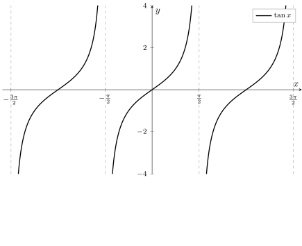
The functions $\sin x$ and $\cos x$ are periodic with period $2\pi$ and take values in $[-1,1]$. They arise as the coordinates of a point moving along the unit circle, hence their repetitive, wave-like character. The function $\tan x=\tfrac{\sin x}{\cos x}$ has vertical asymptotes wherever the cosine vanishes.

Sine and cosine are the same shape shifted by $\tfrac{\pi}{2}$, with period $2\pi$ and values in $[-1,1]$.

Tangent with vertical asymptotes — The tangent $\tan x=\tfrac{\sin x}{\cos x}$ has vertical asymptotes at the points where $\cos x=0$, that is, every $\pi$.

Properties of functions

The properties below describe the behaviour of a function independently of its formula and form the basis for analysing models.

Monotonicity

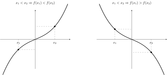
A function is increasing when it preserves the order of arguments, and decreasing when it reverses it:

increasing: if $x_1 \lt x_2$, then $f(x_1) \lt f(x_2)$;
decreasing: if $x_1 \lt x_2$, then $f(x_1) \gt f(x_2)$.

An increasing and a decreasing function — An increasing function preserves the order of arguments (a larger argument gives a larger value); a decreasing function reverses it.

Extrema

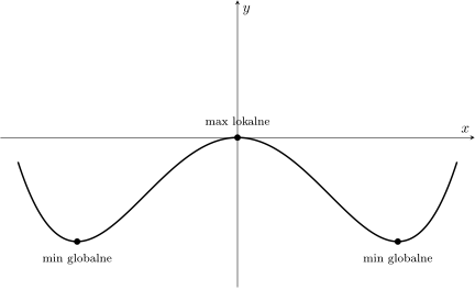
A maximum and a minimum are points at which the function locally attains its greatest or least value. We distinguish local extrema (highest or lowest in some neighbourhood) and global ones (over the whole domain). This notion is central to the least squares method, which seeks the minimum of the sum of squared residuals.

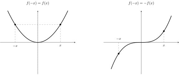
Parity

Even: $f(-x)=f(x)$ — symmetry about the vertical axis (e.g. $x^2$).
Odd: $f(-x)=-f(x)$ — symmetry about the origin (e.g. $x^3$).

An even and an odd function — An even function is a mirror image about the vertical axis; an odd function is symmetric about the origin.

Periodicity

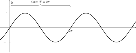
A function is periodic when its graph repeats over a fixed segment $T$ (the period): $f(x+T)=f(x)$ for all $x$. The classic example is the sine with period $2\pi$ — the basis of seasonality models in time series.

Convexity and concavity

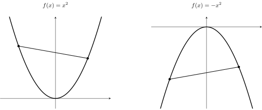
Convex: the chord joining two points of the graph lies above the graph (e.g. $x^2$).
Concave: the chord lies below the graph (e.g. $-x^2$, $\ln x$).

Convexity decides whether a point where the derivative vanishes is a minimum or a maximum, and guarantees uniqueness of the solution in optimisation problems — which makes it a concept central to estimation.

A convex and a concave function with chords — For a convex function the chord between two points runs above the curve; for a concave function it runs below it.

Asymptotes

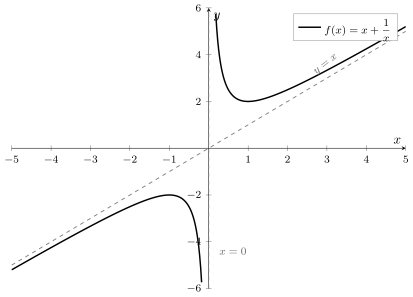
An asymptote is a line that the graph approaches without bound. It may be vertical (the function tends to $\pm\infty$), horizontal, or oblique.

Graph transformations

Knowing the graph of a function $f$, one can directly draw a whole family of derived functions by shifts and reflections.

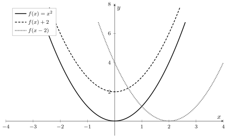
Shifts. Adding a constant to the value, $f(x)+a$, shifts the graph vertically; the substitution $f(x-a)$ shifts it horizontally by $a$ to the right (for $a\gt 0$).

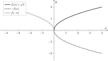
Shifts of a function graph — The expression $f(x)+2$ raises the parabola by $2$, and $f(x-2)$ shifts it $2$ to the right. The shape is unchanged.

Reflections. Changing the sign of the value, $-f(x)$, reflects the graph about the horizontal axis; changing the sign of the argument, $f(-x)$, reflects it about the vertical axis.

Reflections of a function graph — The expression $-f(x)$ gives a reflection about the horizontal axis, and $f(-x)$ about the vertical axis. From a single graph of $\sqrt{x}$, three arise in this way.

Composition of functions

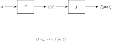
Given two functions $f$ and $g$, their composition is the function $(f\circ g)(x)=f\big(g(x)\big)$: first $g$ acts, and $f$ acts on its result. For the composition to make sense, the values of $g$ must belong to the domain of $f$.

Example

Evaluating a composition

Let $g(x)=x+1$ and $f(u)=u^2$. Then for $x=3$

$$ (f\circ g)(3)=f\big(g(3)\big)=f(4)=16. $$

Order matters: $(g\circ f)(3)=g\big(f(3)\big)=g(9)=10\ne 16$. In general $f\circ g\ne g\circ f$.

Composition of functions on concrete numbers — Composition $f\circ g$ on concrete numbers: the argument $x=3$ passes through $g$ (giving $4$), and the result enters $f$ as input (giving $16$). Two rules act in series.

Composition of functions as two machines in series — Composition as two machines connected in series: the output of the first becomes the input of the second.

The inverse function

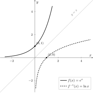
The inverse function $f^{-1}$ undoes the action of $f$: if $f(a)=b$, then $f^{-1}(b)=a$. Geometrically, the graph of the inverse is the reflection of the graph of $f$ about the line $y=x$, because swapping the roles of argument and value is precisely a swap of coordinates.

The exponential function and the logarithm as a reflection about y=x — The graph of the inverse function is a mirror image of the graph of $f$ about the line $y=x$. The point $(a,b)$ on the graph of $f$ corresponds to the point $(b,a)$ on the graph of $f^{-1}$.

Condition for the existence of an inverse.

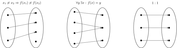
A function can be inverted only when it is one-to-one (an injection) — distinct arguments correspond to distinct values. Otherwise the inverse assignment would not be single-valued.

Injection, surjection, bijection

Injection (one-to-one): distinct arguments correspond to distinct values.
Surjection (“onto”): every value of the codomain is attained by some argument.
Bijection: both an injection and a surjection — a perfect one-to-one pairing. Only a bijection guarantees the existence of an inverse over the whole codomain.

Injection, surjection, and bijection — Three types of mappings: an injection (distinct values), a surjection (covers the whole set $Y$), a bijection (a perfect one-to-one pairing). The panels are characterised by the formulas above them.

Functions of several variables (3D)

So far a function had a single input. In econometrics there are almost always several: a function $z=f(x,y)$ assigns to a pair of numbers $(x,y)$ a single value $z$, which geometrically gives a surface in three-dimensional space. This is the natural language of multiple regression, production functions, and utility functions.

Paraboloid and saddle

The surface $z=x^2+y^2$ is a paraboloid — a “bowl” with a single minimum in the centre, exactly like the sum of squared residuals in OLS. The surface $z=x^2-y^2$ is a saddle: in one direction it rises, in the other it falls, so its centre is neither a minimum nor a maximum.

Paraboloid z = x squared plus y squared — The paraboloid $z=x^2+y^2$ — a “bowl” with a single minimum. This is the geometry minimised by the least squares method.

Saddle surface z = x squared minus y squared — The saddle $z=x^2-y^2$ — up along one axis, down along the other. A saddle point can be a trap for optimisation algorithms.

Level curves — a bridge between 3D and 2D

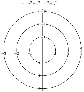
A three-dimensional surface can be represented in the plane by means of level curves: curves along which the function takes a constant value, $f(x,y)=c$. This is the same principle by which terrain-relief maps are drawn. For the paraboloid $z=x^2+y^2$ the level curves $x^2+y^2=c$ are circles of radius $\sqrt{c}$ — the higher up the bowl, the larger the circle.

Level curves of a paraboloid as concentric circles — Level curves of the paraboloid $z=x^2+y^2$: the curves of constant value $x^2+y^2=c$ are concentric circles. They allow a three-dimensional surface to be represented on a flat drawing.

Wave and two-dimensional bell

The surface $z=\sin x\,\cos y$ forms a regular wave, and $z=e^{-(x^2+y^2)/2}$ is a two-dimensional Gaussian bell — the density graph of the multivariate normal distribution.

Wave surface z = sin x cos y — The wave $z=\sin x\cos y$ — the product of two periodic functions yields a regular lattice of crests and troughs.

The regression plane and the Cobb-Douglas function

Two surfaces connect mathematics with economics. The plane $z=\beta_0+\beta_1 x+\beta_2 y$ is a regression model with two explanatory variables — OLS fits it so that it lies closest to the cloud of observations. The Cobb-Douglas production function $z=x^{\alpha}y^{\beta}$ describes how inputs (e.g. labour and capital) translate into the volume of output.

Regression plane with a point cloud — The plane $z=0.5x+0.3y+1$ fitted to a cloud of observations — this is what regression with two explanatory variables looks like. It is the three-dimensional counterpart of the regression line.

The Cobb-Douglas production function $z=\sqrt{x\,y}$: it grows with each input, but ever more slowly, corresponding to diminishing marginal returns.

The idea of the fourth dimension and the space $\mathbb{R}^n$

A function $z=f(x,y)$ lives in three-dimensional space, which can be drawn directly. But what happens when there are three, four, or more explanatory variables? Formally we encounter no difficulty whatsoever: the function

$$ f\colon \mathbb{R}^n \to \mathbb{R}, \qquad y=f(x_1,x_2,\dots,x_n), $$

assigns to a tuple of $n$ numbers a single value. The difficulty is purely visual — paper and screen have only two dimensions, and our spatial imagination reaches three. There are, however, ways to make the idea of higher dimensions tangible.

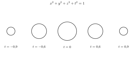
First way — slices (layer by layer). A four-dimensional object can be viewed as a film: for each value of the fourth coordinate $t$ we obtain a three-dimensional slice, and successive slices form a sequence. The four-dimensional sphere $x^2+y^2+z^2+t^2=1$ appears at $t=-1$ as a point, swells to a full ball at $t=0$, and vanishes at $t=1$ — just as a three-dimensional ball, cut by a plane, yields a growing and shrinking disc.

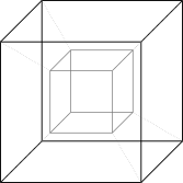
Slices of a hypersphere at successive instants as the idea of the fourth dimension — The fourth dimension as a film: successive three-dimensional slices of the 3-sphere $x^2+y^2+z^2+t^2=1$ at instants $t$. The radius of the slice is $\sqrt{1-t^2}$ — the figure emerges from a point, grows to a full ball, and vanishes. This is how, “layer by layer,” we experience a dimension that cannot be drawn all at once.

Second way — projection (shadow). Just as a three-dimensional cube casts a two-dimensional shadow onto the plane, a four-dimensional cube (a tesseract) casts a three-dimensional shadow. In the figure below we represent that shadow as a “cube within a cube”: the edges joining the inner cube to the outer one correspond to a displacement along the fourth axis. The inner cube is not really smaller — it appears smaller because it is farther away in a direction we cannot see.

Projection of a tesseract as a cube within a cube — The shadow of a tesseract (4-cube): a three-dimensional projection shown as a cube inscribed in a cube. The dotted edges join the two cubes and correspond to a displacement along the fourth axis — a direction that cannot be drawn directly.

Generalisation to $\mathbb{R}^n$.

Concepts from one and two variables carry over to any dimension without change of substance. A point $(x_1,\dots,x_n)$ is an element of $\mathbb{R}^n$; the level set $f=c$ becomes a hypersurface; the minimum of a function corresponds to the “lowest” point of an $n$-dimensional bowl. The rules of calculus remain the same — only the number of coordinates changes. This is why a regression model with many variables, though invisible, obeys exactly the same laws as a line and a plane.

Significance for econometrics.

An econometric model is a function. Simple regression is a line, regression with two variables is a plane, and regression with many variables is a hypersurface in $\mathbb{R}^n$ that cannot be drawn but is governed by the same rules. Understanding functions — the domain, monotonicity, convexity, and extrema — is a prerequisite for understanding estimation and optimisation.

Application — case study: market equilibrium

A classic economic application of functions is the model of market equilibrium, in which demand and supply are functions of price. Consider a market for a good described by the demand function $P_D=20-0.5Q$ (the lower the price, the larger the quantity bought) and the supply function $P_S=5+0.25Q$ (the higher the price, the larger the quantity offered), where $Q$ is quantity in thousands of units and $P$ the price.

The equilibrium point is the argument for which both functions take the same value — geometrically the intersection of the graphs. Setting them equal:

$$ 20-0.5Q=5+0.25Q \;\Longrightarrow\; 15=0.75Q \;\Longrightarrow\; Q^\*=20,\qquad P^\*=20-0.5\cdot 20=10. $$

The market clears at a price of $10$ and a quantity of $20$ thousand units. This is precisely an application of the intermediate value theorem: excess demand $P_D-P_S$ is positive at low prices and negative at high prices, and being a continuous function, it must vanish somewhere — and that is where the equilibrium price lies.

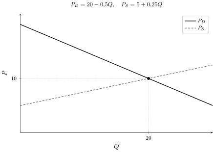
Market equilibrium — intersection of demand and supply functions — Market equilibrium as the intersection of the demand and supply functions. The decreasing demand function $P_D=20-0.5Q$ and the increasing supply function $P_S=5+0.25Q$ intersect at the point $(Q^\*,P^\*)=(20;10)$ — the equilibrium price and quantity.

This simple model captures the essence of econometric thinking: economic phenomena are written as functions, and their properties (monotonicity, point of intersection, slope) carry economic meaning — the slope of the demand function relates to price elasticity, and the intersection determines the state toward which the market tends.