Integrals — summing infinitely many terms

Abstract

The integral built from the ground up: genesis (Archimedes' method of exhaustion, the problem of area, Newton and Leibniz), the Riemann sum with lower and upper sums, the definite integral as area, the antiderivative and the indefinite integral, the fundamental theorem of calculus with justification, integration by substitution and by parts (with geometric interpretation), improper integrals, economic applications (total cost, consumer surplus, present value), double integrals as volume in 3D, and the generalisation to ℝⁿ. Every concept and every example with its own figure.

If the derivative measures the rate of change, then the integral measures accumulation — a sum of infinitely many infinitely small increments. Geometrically it is the area under a graph; in economics it is the total cost summed from the marginal cost, consumer surplus, or the present value of a stream of payments. This chapter builds the notion of the integral from the historical problem of area, through the Riemann sum and the fundamental theorem of calculus, up to improper integrals and multiple integrals in the space $\mathbb{R}^n$. Every concept and every example is given its own figure.

The genesis of the concept of an integral

The integral is historically older than the derivative. As early as the third century BC, Archimedes determined the areas of curvilinear figures by the method of exhaustion: he inscribed ever-finer polygons (or rectangles) in a figure, whose total area grew and approached the area of the figure. By this route he proved that the area of a parabolic segment is exactly $\tfrac{4}{3}$ of the area of the triangle inscribed in it — a result reached two millennia later by a one-line integral computation.

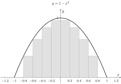
Area under a parabola approximated by inscribed rectangles — Archimedes’ method of exhaustion: the area under the parabola $y=1-x^2$ is approximated by the sum of the areas of inscribed rectangles. The finer the partition, the closer to the exact value. This is the prototype of the definite integral.

Archimedes’ method was ingenious, but each case required fresh inventiveness. The breakthrough came in the seventeenth century, when Isaac Newton and Gottfried Wilhelm Leibniz discovered that the area under a graph and the slope of the tangent are mutually inverse operations — what we now call the fundamental theorem of calculus. From then on, area is computed not by laborious summation but by reversing differentiation. A rigorous definition of area itself was given in the nineteenth century by Bernhard Riemann, and it is where we begin.

The Riemann sum and the definite integral

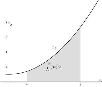
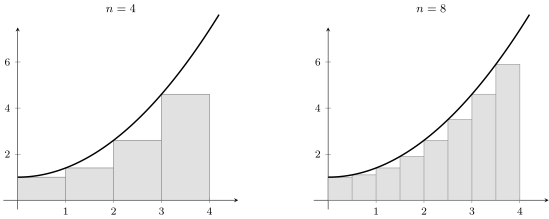
To define the area under the graph of a function $f$ on an interval $[a,b]$, we divide the interval into $n$ pieces of width $\Delta x$, choose a point $x_i^*$ in each, and approximate the area by the sum of the areas of rectangles of heights $f(x_i^*)$.

Definition

The definite integral (Riemann)

The definite integral of a function $f$ on an interval $[a,b]$ is the limit of the Riemann sums as the partition is refined without bound:

$$ \int_a^b f(x)\,dx=\lim_{n\to\infty}\sum_{i=1}^{n}f(x_i^*)\,\Delta x, $$

provided this limit exists and does not depend on the partition or the choice of the points $x_i^*$. Geometrically it is the area enclosed between the graph, the horizontal axis, and the lines $x=a$ and $x=b$.

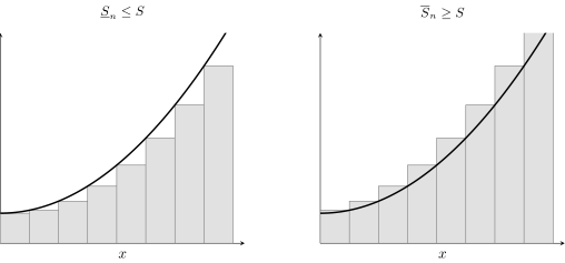
The integral as the area under a graph — The definite integral $\int_a^b f(x)\,dx$ is the area enclosed between the graph of the function, the horizontal axis, and the vertical lines $x=a$ and $x=b$.

That the limit exists and is independent of the details of the partition is seen from trapping the area between two approximations. The lower sum uses the smallest value of the function on each piece (the rectangles fit under the graph), the upper sum the largest (the rectangles protrude above). The true area always lies between them, and both sums converge to a common value as the partition is refined.

Lower and upper sums trapping the area under a graph — The lower sum (left) lies under the graph, the upper sum (right) above it. The true area is between them. As the partition is refined, both sums converge to a common limit — the value of the integral.

Riemann sums — approximating area by rectangles — The more (and narrower) the rectangles, the more accurate the approximation of the area. As $n\to\infty$ the Riemann sum tends to the exact value of the integral.

The antiderivative and the indefinite integral

Computing the limit of Riemann sums each time would be laborious. The key lies in the notion inverse to the derivative.

Definition

Antiderivative and indefinite integral

An antiderivative of a function $f$ is any function $F$ such that $F'(x)=f(x)$. If $F$ is an antiderivative, then so is $F+C$ (for any constant $C$), since the derivative of a constant is zero. The set of all antiderivatives is written as the indefinite integral:

$$ \int f(x)\,dx=F(x)+C. $$

The constant $C$ is not an arbitrary addition — it reflects the fact that area measured from different reference levels differs by a constant. Geometrically, all the antiderivatives form a family of curves shifted vertically, having at every point the identical slope $f(x)$.

A family of antiderivatives differing by a constant — The antiderivatives of the function $2x$ form a family of parabolas $x^2+C$ differing only by a vertical shift. At every point they have the identical slope, hence the same derivative $2x$.

Theorem

Basic integration formulas

$$ \int x^n\,dx=\frac{x^{n+1}}{n+1}+C\ (n\ne -1),\quad \int\frac{1}{x}\,dx=\ln|x|+C,\quad \int e^x\,dx=e^x+C, $$

$$ \int a^x\,dx=\frac{a^x}{\ln a}+C,\quad \int\sin x\,dx=-\cos x+C,\quad \int\cos x\,dx=\sin x+C. $$

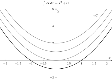
Each of these formulas is simply the reversal of the corresponding differentiation rule.

For example $\int x^3\,dx=\tfrac{x^4}{4}+C$, because $\big(\tfrac{x^4}{4}\big)'=x^3$.

The fundamental theorem of calculus

This theorem binds together the two poles of analysis — differentiation and integration — making them mutually inverse operations.

Theorem

The fundamental theorem of calculus

Let $f$ be continuous on $[a,b]$. Then:

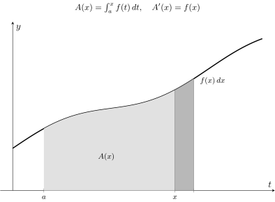
(part I) the area function $A(x)=\displaystyle\int_a^x f(t)\,dt$ is differentiable and $A'(x)=f(x)$;

(part II) for any antiderivative $F$ (where $F'=f$),

$$ \int_a^b f(x)\,dx=F(b)-F(a). $$

Proof

Part I: the derivative of the area function

Increment of area. The difference $A(x+h)-A(x)$ is the area of a narrow strip over the interval $[x,x+h]$.
Estimating the strip. For small $h$ the strip is nearly a rectangle of base $h$ and height $f(x)$, so $A(x+h)-A(x)\approx f(x)\,h$. More precisely, by the continuity of $f$ the height of the strip lies between the extrema of $f$ on $[x,x+h]$, both of which tend to $f(x)$.
Difference quotient. Hence $\dfrac{A(x+h)-A(x)}{h}\to f(x)$ as $h\to 0$, i.e. $A'(x)=f(x)$.
Conclusion (part II). Since $A$ and $F$ have the same derivative $f$, they differ by a constant; the increment $A(b)-A(a)=\int_a^b f$ thus equals $F(b)-F(a)$. $\;$

∎

The area function and a narrow strip illustrating the fundamental theorem — The idea of the proof: the area function $A(x)$ accumulates the area from $a$ to $x$. Adding a narrow strip of width $dx$ increases the area by about $f(x)\,dx$, so the rate of growth of the area is $A'(x)=f(x)$ — integration and differentiation are inverse operations.

Thanks to this theorem we compute the definite integral without Riemann sums. For example

$$ \int_0^3 x^2\,dx=\Big[\frac{x^3}{3}\Big]_0^3=\frac{27}{3}-0=9. $$

Methods of integration

Integration by substitution

This method reverses the chain rule. If the integrand contains a function and its derivative, we substitute $u=g(x)$, whence $du=g'(x)\,dx$.

Example

Substitution

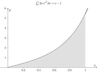
In the integral $\displaystyle\int 2x\,e^{x^2}\,dx$ we take $u=x^2$, so $du=2x\,dx$:

$$ \int 2x\,e^{x^2}\,dx=\int e^u\,du=e^u+C=e^{x^2}+C. $$

For the definite version $\displaystyle\int_0^1 2x\,e^{x^2}\,dx=\big[e^{x^2}\big]_0^1=e-1\approx 1.718$.

Area under the integrand under substitution — The integral $\int_0^1 2x\,e^{x^2}\,dx$ is the area under the integrand on $[0,1]$. The substitution $u=x^2$ reduces it to the elementary $\int e^u\,du$, giving the value $e-1$.

Integration by parts

This method reverses the product rule. From $(uv)'=u'v+uv'$, after integration we obtain

$$ \int u\,dv=uv-\int v\,du. $$

We use it when the integrand is a product of functions of different types (e.g. a polynomial and an exponential).

Example

By parts

In the integral $\displaystyle\int x\,e^x\,dx$ we take $u=x$ and $dv=e^x\,dx$, whence $du=dx$ and $v=e^x$:

$$ \int x\,e^x\,dx=x e^x-\int e^x\,dx=x e^x-e^x+C=e^x(x-1)+C. $$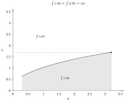

A rectangle's area split into two integrals — integration by parts — The geometric meaning of integration by parts. For an increasing curve $v(u)$, the area of the rectangle $uv$ splits into two parts: the area under the curve $\int v\,du$ and the area beside it $\int u\,dv$. Hence $\int u\,dv=uv-\int v\,du$.

Improper integrals

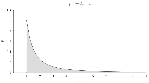
The integral can be extended to infinite intervals by treating it as a limit. Surprisingly, the area under an infinitely long tail can be finite:

$$ \int_1^{\infty}\frac{1}{x^2}\,dx=\lim_{b\to\infty}\Big[-\frac{1}{x}\Big]_1^b=\lim_{b\to\infty}\Big(1-\frac{1}{b}\Big)=1. $$

This convergence underlies the present value of a perpetuity: an infinite stream of decreasing, discounted payments sums to a finite amount.

A finite area under an infinite tail of a function — The improper integral $\int_1^{\infty}\tfrac{1}{x^2}\,dx$: although the region stretches to infinity, its area is finite and equal to $1$. This is the mathematical basis for the finite valuation of an infinite stream of payments.

Applications in economics

Total cost from marginal cost

Since marginal cost $MC(Q)$ is the derivative of total cost, total cost is its integral. For $MC(Q)=3Q^2-4Q+5$ and fixed cost $FC=100$:

$$ TC(Q)=100+\int_0^Q(3q^2-4q+5)\,dq=100+Q^3-2Q^2+5Q. $$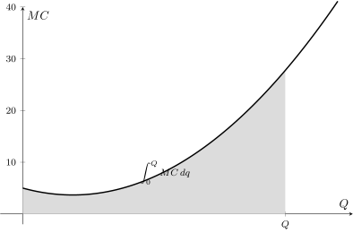

Total cost as the area under the marginal cost curve — Variable total cost is the area under the marginal cost curve $MC(Q)$. Integration sums the cost of each successive unit of output.

Consumer surplus

Consumer surplus is the difference between what buyers would be willing to pay and what they actually pay — geometrically the area between the demand curve and the market price. For demand $Q=100-2P$ and price $P^*=20$ (whence $Q^*=60$) we invert demand to $P=50-\tfrac{Q}{2}$ and integrate:

$$ CS=\int_0^{60}\Big(50-\frac{Q}{2}-20\Big)\,dQ=\Big[30Q-\frac{Q^2}{4}\Big]_0^{60}=1800-900=900. $$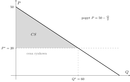

Consumer surplus as the area under the demand curve — Consumer surplus is the area between the demand curve and the market price $P^*$ — the total “bonus” of all buyers who would pay more than they actually do. Here $CS=900$.

Present value of a continuous stream

For a continuous stream of payments $\pi(t)$ at a discount rate $r$, the net present value is

$$ NPV=\int_0^T \pi(t)\,e^{-rt}\,dt, $$

which is the continuous counterpart of the discrete sum $\sum_{t=0}^{T}\tfrac{\pi_t}{(1+r)^t}$. The continuous form is analytically more convenient and connects with the limit defining continuous compounding.

Multiple integrals and the space $\mathbb{R}^n$

Just as the single integral sums the areas of strips, giving the area under a curve, the double integral sums the volumes of columns, giving the volume under a surface:

$$ \iint_D f(x,y)\,dx\,dy. $$

The double integral as the volume under a surface — The double integral $\iint_D f(x,y)\,dx\,dy$ is the volume of the solid under the surface $z=f(x,y)$ over the region $D$ — a generalisation of the “area under a curve” one dimension higher.

Integrals in $\mathbb{R}^n$ and the fourth dimension.

The Riemann-sum construction generalises to any dimension: the single integral sums over segments, the double over rectangles, the triple $\iiint f\,dx\,dy\,dz$ over cubes, and the $n$-fold $\int_{\mathbb{R}^n} f\,d\mathbf{x}$ over $n$-dimensional cubes. The result in $\mathbb{R}^4$ and higher cannot be drawn as a “solid,” but the computation is the same — we sum infinitely many infinitely small elements. In statistics such integrals give the probability mass: the integral of a density over a region in $\mathbb{R}^n$ is the probability that the vector of random variables falls in that region. A four-dimensional integral can be computed “layer by layer,” fixing one variable and integrating over three-dimensional slices (Fubini’s theorem).

Application — case study: net present value of an investment (NPV)

An investment generates a continuous stream of revenue — approximately $100$ thousand per year for $10$ years. At a discount rate $r=8\%$, revenue received at time $t$ is worth $100\,e^{-0.08t}$ today (continuous discounting, see limits). The total present value of this stream is given by an integral:

$$ \mathrm{NPV}_{\text{revenue}}=\int_0^{10}100\,e^{-0.08t}\,dt=100\cdot\Big[-\tfrac{1}{0.08}e^{-0.08t}\Big]_0^{10}=1250\big(1-e^{-0.8}\big)\approx 688\ \text{thousand}. $$

If the initial outlay is $500$ thousand, the project’s net present value is $688-500=188$ thousand $\gt 0$ — the investment is profitable. Geometrically, NPV is the area under the discounted revenue curve.

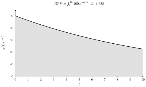
NPV as the area under the discounted revenue curve — The present value of a continuous revenue stream is the area under the curve $100\,e^{-0.08t}$ on the interval $[0,10]$. Discounting makes distant revenue weigh less; the integral sums it all, giving $\mathrm{NPV}\approx 688$ thousand.

This case study shows why the integral is indispensable in finance: summing infinitely many instantaneous, decreasingly discounted revenues is exactly the operation of integration, and the result decides the profitability of a decision.

Integrals — summing infinitely many terms

The genesis of the concept of an integral

The Riemann sum and the definite integral

The antiderivative and the indefinite integral

The fundamental theorem of calculus

Methods of integration

Integration by substitution

Integration by parts

Improper integrals

Applications in economics

Total cost from marginal cost

Consumer surplus

Present value of a continuous stream

Multiple integrals and the space $\mathbb{R}^n$

Application — case study: net present value of an investment (NPV)

Further reading

Summary