Linear algebra — vectors and matrices
Linear algebra built from the ground up: genesis (systems of equations, Gaussian elimination, Cayley's matrices, determinants), vectors and their operations, the dot product, norm and angle, linear combination and basis, matrices and multiplication with a full computation, the matrix as a linear transformation, the determinant as area, the inverse matrix, eigenvalues and eigenvectors, the geometry of systems of equations, regression in matrix notation and orthogonal projection in 2D and 3D, and the generalisation to ℝⁿ. Every concept and every example with its own figure.
Linear algebra is the language in which all of econometrics is written. The regression model — regardless of the number of variables — reduces to a single matrix formula $\hat{\boldsymbol\beta}=(\mathbf{X}^\top\mathbf{X})^{-1}\mathbf{X}^\top\mathbf{y}$, and understanding it requires the calculus of vectors and matrices. This chapter builds that calculus from the ground up: from the genesis of the concept, through vectors, matrices, and their geometric meaning, up to eigenvalues and orthogonal projection in the space $\mathbb{R}^n$. Every concept and every example is given its own figure.
The genesis of linear algebra
Linear algebra grew out of the most practical of problems — solving systems of linear equations. As early as the ancient Chinese Nine Chapters on the Mathematical Art (c. 2nd century BC), the coefficients of a system were written in a rectangular array and transformed into a form from which the solution could be read off — this was in fact the elimination method we now call Gaussian elimination. In the seventeenth and eighteenth centuries Leibniz and Cramer introduced determinants as a tool for deciding the existence of a solution. The term “matrix” itself is due to James Sylvester (1850), and the matrix calculus — operations, multiplication, inversion — was systematised by Arthur Cayley in 1858. The notion of a vector matured in parallel, in the work of Hamilton and Grassmann on quantities possessing direction. From these two currents — equations and directed quantities — arose a unified theory, which we begin with the vector.
Vectors
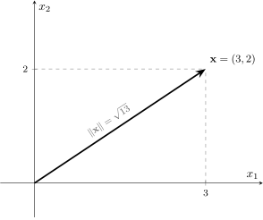
A vector is an ordered list of numbers (coordinates), usually written in a column:
$$ \mathbf{x}=\begin{pmatrix}x_1\\x_2\\\vdots\\x_n\end{pmatrix}. $$Geometrically a vector in $\mathbb{R}^2$ or $\mathbb{R}^3$ is an arrow from the origin to the point with the given coordinates.
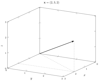
Vectors also make sense in three and more dimensions. An arrow in $\mathbb{R}^3$ has three coordinates, and its projections onto the axes determine a “box” whose diagonal is the vector itself.
Operations on vectors
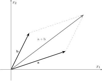
Addition and multiplication by a number are performed coordinate-wise:
$$ \mathbf{a}+\mathbf{b}=(a_1+b_1,\dots,a_n+b_n),\qquad c\,\mathbf{a}=(ca_1,\dots,ca_n). $$Geometrically, addition corresponds to placing one arrow at the tip of the other — the sum is the diagonal of the parallelogram spanned by the two vectors.
Dot product, norm, and angle
The dot product of two vectors is the sum of the products of corresponding coordinates:
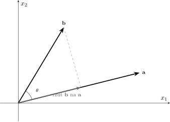
$$ \mathbf{a}\cdot\mathbf{b}=\sum_{i=1}^{n}a_i b_i. $$The norm (length) of a vector is $\|\mathbf{x}\|=\sqrt{\mathbf{x}\cdot\mathbf{x}}=\sqrt{x_1^2+\dots+x_n^2}$. The dot product is related to the angle between the vectors by $\mathbf{a}\cdot\mathbf{b}=\|\mathbf{a}\|\,\|\mathbf{b}\|\cos\theta$.
From the last formula follows a key conclusion: two nonzero vectors are perpendicular (orthogonal) exactly when their dot product is zero (because $\cos 90°=0$). This equivalence is the foundation of the geometry of the least squares method.
Linear combination, span, and basis
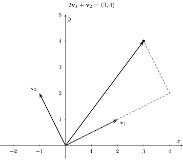
Combining addition and multiplication by a number, we form a linear combination of vectors: $c_1\mathbf{v}_1+c_2\mathbf{v}_2+\dots$. The set of all such combinations is called the span of these vectors. Two non-collinear vectors span the whole plane — every point of it can be reached as their unique combination. Such a minimal set of vectors spanning the space is a basis.
Matrices
Matrix multiplication
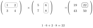
The product $\mathbf{C}=\mathbf{A}\mathbf{B}$ (where $\mathbf{A}$ is $m\times k$ and $\mathbf{B}$ is $k\times n$) has entries that are dot products of the rows of $\mathbf{A}$ with the columns of $\mathbf{B}$:
$$ c_{ij}=\sum_{l=1}^{k}a_{il}\,b_{lj}. $$The inner dimensions must match ($k=k$), and the result has the outer dimensions $m\times n$. Matrix multiplication is not commutative: in general $\mathbf{AB}\ne\mathbf{BA}$.
The top-right entry is the dot product of the first row with the second column: $1\cdot 6+2\cdot 8=22$. The remaining entries are computed analogously.
The matrix as a linear transformation
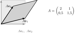
The deepest meaning of a matrix is geometric: a matrix $\mathbf{A}$ transforms every vector $\mathbf{x}$ into a new vector $\mathbf{A}\mathbf{x}$, deforming the whole space in a linear way. To understand such a transformation, it is enough to know where the basis vectors go — the rest follows from linearity.
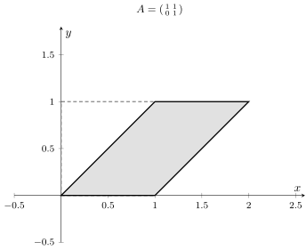
A concrete example is the shear: the matrix $\bigl(\begin{smallmatrix}1&1\\0&1\end{smallmatrix}\bigr)$ leaves the horizontal axis unchanged but pushes the top edge sideways, turning the square into a slanted parallelogram.
The determinant
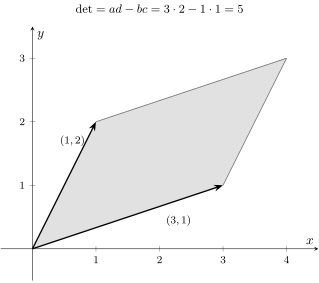
The determinant of a square matrix measures how many times the transformation changes area (in 2D) or volume (in 3D). For a $2\times 2$ matrix
$$ \det\begin{pmatrix}a&b\\c&d\end{pmatrix}=ad-bc. $$The absolute value of the determinant is the area of the parallelogram spanned by the columns; the sign tells the orientation. A zero determinant means the transformation “flattens” the space (the columns are collinear) — the matrix is then non-invertible.
The inverse matrix
The identity matrix $\mathbf{I}$ (ones on the diagonal, zeros elsewhere) satisfies $\mathbf{AI}=\mathbf{IA}=\mathbf{A}$ — it is the counterpart of the number $1$. The inverse matrix $\mathbf{A}^{-1}$ is one such that $\mathbf{A}\mathbf{A}^{-1}=\mathbf{A}^{-1}\mathbf{A}=\mathbf{I}$; it exists only for square matrices with a nonzero determinant. For $2\times 2$:
$$ \begin{pmatrix}a&b\\c&d\end{pmatrix}^{-1}=\frac{1}{ad-bc}\begin{pmatrix}d&-b\\-c&a\end{pmatrix}. $$Dividing by $ad-bc$ explains why a zero determinant makes inversion impossible — the transformation irreversibly loses a dimension.
Eigenvalues and eigenvectors
Some vectors, under the action of a matrix, do not change direction — they are merely stretched or compressed. Such a vector is an eigenvector, and the stretching factor an eigenvalue.
A nonzero vector $\mathbf{v}$ is an eigenvector of a matrix $\mathbf{A}$ if
$$ \mathbf{A}\mathbf{v}=\lambda\,\mathbf{v} $$for some number $\lambda$ — the eigenvalue. Multiplication by $\mathbf{A}$ acts on $\mathbf{v}$ like ordinary scaling.
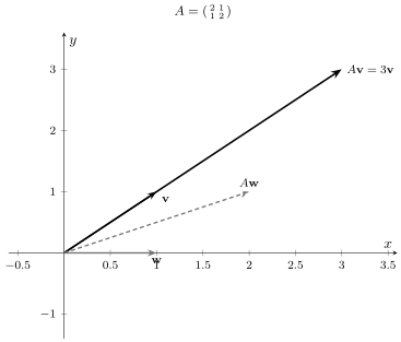
Eigenvalues describe the “natural axes” of a transformation and are central to principal component analysis (PCA), the study of model stability, and the structure of the covariance matrix.
The geometry of systems of equations
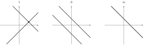
A system of two linear equations in two unknowns is geometrically two lines in the plane. The number of solutions depends on their mutual position: intersecting lines give one solution, parallel lines give none, and coincident lines give infinitely many. The same classification holds in higher dimensions (planes in $\mathbb{R}^3$ and beyond) and explains when a model has a unique solution.
Regression in matrix notation
The entire linear regression model is written in matrix form regardless of the number of variables. Given $n$ observations and $k$ explanatory variables, we arrange the data matrix $\mathbf{X}$ of dimension $n\times(k+1)$ (the first column is ones for the intercept), the parameter vector $\boldsymbol\beta$, and the observation vector $\mathbf{y}$. The model and its solution are
$$ \mathbf{y}=\mathbf{X}\boldsymbol\beta+\boldsymbol\varepsilon,\qquad \hat{\boldsymbol\beta}=(\mathbf{X}^\top\mathbf{X})^{-1}\mathbf{X}^\top\mathbf{y}. $$The estimator $\hat{\boldsymbol\beta}$ minimises $\|\mathbf{y}-\mathbf{X}\boldsymbol\beta\|^2$ — the squared norm of the residual vector, i.e. the sum of squared deviations. The full derivation of this formula is presented in the chapter on the least squares method.
Geometry: the orthogonal projection
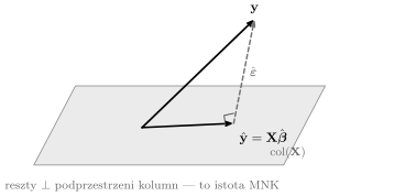
Why the orthogonal projection is best.
The columns of the matrix $\mathbf{X}$ span a certain subspace $\mathrm{col}(\mathbf{X})$. The observation vector $\mathbf{y}$ usually does not lie in it. The best fit $\hat{\mathbf{y}}=\mathbf{X}\hat{\boldsymbol\beta}$ is the orthogonal projection of $\mathbf{y}$ onto this subspace, because it minimises the distance. The residual vector $\hat{\boldsymbol\varepsilon}=\mathbf{y}-\hat{\mathbf{y}}$ is then perpendicular to the subspace — if it were not, it could be shortened, and the fit would not be best. The perpendicularity condition $\mathbf{X}^\top\hat{\boldsymbol\varepsilon}=\mathbf{0}$ is precisely the normal equations.
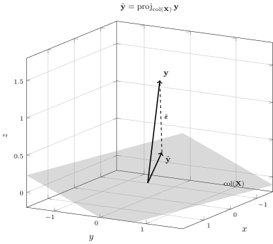
Linear algebra in $\mathbb{R}^n$.
Every concept of this chapter — vector, dot product, perpendicularity, projection — carries over unchanged to any dimension. In regression the vectors $\mathbf{y}$, $\hat{\mathbf{y}}$, and the residuals live in a space $\mathbb{R}^n$ with as many dimensions as there are observations (often thousands). This space cannot be drawn, but the rules remain identical to those in the plane and in space: the orthogonal projection minimises the distance, and the perpendicularity of the residuals to the columns of $\mathbf{X}$ defines the OLS estimator. This is precisely the power of linear algebra — a single notation and a single geometry work in every dimension, regardless of whether we can draw them.
Application — case study: the Markowitz portfolio
The best-known economic application of linear algebra is Harry Markowitz’s portfolio theory (Nobel Prize 1990). An investor splits capital between two assets with returns and risk: A ($\mu_A=6\%$, $\sigma_A=10\%$) and B ($\mu_B=12\%$, $\sigma_B=20\%$), correlated with coefficient $\rho=0.2$. The weights $w$ and $1-w$ determine a portfolio whose variance is written as a quadratic form with the covariance matrix:
$$ \sigma_p^2=\mathbf{w}^\top\boldsymbol\Sigma\,\mathbf{w}=w^2\sigma_A^2+(1-w)^2\sigma_B^2+2w(1-w)\,\rho\sigma_A\sigma_B. $$The minimum-risk portfolio is found by setting the derivative to zero (the condition from the chapter on derivatives):
$$ w^\*=\frac{\sigma_B^2-\rho\sigma_A\sigma_B}{\sigma_A^2+\sigma_B^2-2\rho\sigma_A\sigma_B}=\frac{0.04-0.004}{0.05-0.008}\approx 0.857. $$The optimal portfolio is thus $\approx 85.7\%$ asset A and $14.3\%$ asset B, with risk $\sigma_p\approx 9.6\%$ and return $\mu_p\approx 6.9\%$ — lower risk than either asset alone. This is the effect of diversification, described in the language of the dot product and the covariance matrix.
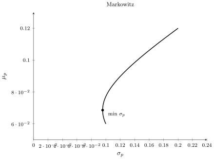
For many assets the weights form a vector $\mathbf{w}\in\mathbb{R}^n$, and the portfolio risk is the quadratic form $\mathbf{w}^\top\boldsymbol\Sigma\mathbf{w}$ — minimisation subject to $\sum w_i=1$ is a classic linear-algebra problem solved with Lagrange multipliers. Thus matrix theory becomes a tool of risk management.
Further reading
Polish textbooks
- A. Białynicki-Birula, Algebra liniowa z geometrią, PWN.
- T. Trzaskalik, Wprowadzenie do badań operacyjnych z komputerem, PWE, Warsaw.
World and economics classics
- G. Strang, Introduction to Linear Algebra, Wellesley-Cambridge Press, 2016.
- S. Axler, Linear Algebra Done Right, Springer, 2015.
Articles
- H. Markowitz, Portfolio Selection, The Journal of Finance 7 (1952), 77–91. DOI: 10.2307/2975974.
Summary
Linear algebra begins with vectors and matrices, but its essence is geometry: a matrix is a transformation of space, the determinant is the scaling of area, eigenvectors are its natural axes, and the orthogonal projection is the best fit. The matrix notation of the regression model and its solution $\hat{\boldsymbol\beta}=(\mathbf{X}^\top\mathbf{X})^{-1}\mathbf{X}^\top\mathbf{y}$ work in a space $\mathbb{R}^n$ of any number of dimensions — hence the universality of this language in econometrics.
Next: Descriptive statistics
- G. Strang, Introduction to Linear Algebra
- 3Blue1Brown — Essence of Linear Algebra
- Python:
A @ B(multiplication),A.T(transpose),np.linalg.inv(A),np.linalg.det(A),np.linalg.eig(A) - R:
A %*% B,t(A),solve(A),det(A),eigen(A)