The Method of Least Squares — A Complete Treatise: History, Theory and Proofs
A comprehensive account of the method of least squares: from the eighteenth-century problem of the figure of the Earth and its precursors (Cotes, Mayer, Bošković), through Legendre's first publication (1805), Gauss's original derivation (1809) and Laplace's probabilistic foundation, to the Gauss-Markov theorem (1823) and the birth of regression — with dates, names, original-language texts, full proofs and portraits.
The method of least squares was not born as an exercise in algebra. It grew out of the most demanding computational problems of the eighteenth and nineteenth centuries — determining the figure of the Earth and the orbits of celestial bodies from observations corrupted by error. This article traces that entire path: from the precursors, through the priority dispute between Legendre and Gauss, to Gauss’s two distinct justifications and the birth of modern regression — with dates, names, original-language texts and full proofs.
Part I. The problem: inconsistent observations (eighteenth century)
In the eighteenth century, astronomy and geodesy posed a difficulty of a new kind. To determine a few unknown quantities — say, the parameters of an orbit, or the flattening of the Earth — practitioners made many measurements, more than there were unknowns. Each measurement was slightly in error, so the resulting system of equations was overdetermined and inconsistent: no single solution satisfied all observations simultaneously.
The figure of the Earth
Newton predicted that the Earth is oblate — flattened at the poles. To settle the matter, the French Academy of Sciences dispatched two expeditions to measure the length of a meridian arc: to Lapland (Maupertuis, 1736–37) and to Peru (Bouguer and La Condamine, 1735–44). From many geodetic measurements, two parameters of the ellipsoid had to be recovered — a classic overdetermined system.
Precursors: the first ways of combining observations
- Roger Cotes (1682–1716) proposed a weighted mean of observations (published posthumously in Harmonia mensurarum, 1722) — the idea of giving greater weight to more precise measurements.
- Tobias Mayer (1723–1762), studying the libration of the Moon (c. 1750), used a “method of averages”: he grouped the equations and summed them, reducing the overdetermined system to a solvable one.
- Ruđer Bošković (1711–1787), measuring a meridian arc near Rome with Christopher Maire (De litteraria expeditione…, 1755), proposed the criterion closest in spirit to least squares: minimise the sum of absolute deviations subject to the constraint that the signed deviations sum to zero — an $L_1$ regression, to which statistics returned only in the twentieth century.
- Leonhard Euler and Pierre-Simon Laplace tried other “methods of combination,” but none was both general and simple.
What was missing was a single, universal principle. It appeared at the start of the nineteenth century — and almost simultaneously in two men.
Part II. Legendre: the first publication (1805)

The first publication of the method was an appendix to Adrien-Marie Legendre’s Nouvelles méthodes pour la détermination des orbites des comètes (1805), entitled Sur la méthode des moindres carrés. It was Legendre who named the method — méthode des moindres carrés — and stated it with disarming clarity:
“De tous les principes qu’on peut proposer pour cet objet, je pense qu’il n’en est pas de plus général, de plus exact, ni d’une application plus facile, que celui dont nous avons fait usage dans les recherches précédentes, et qui consiste à rendre minimum la somme des carrés des erreurs.”
“Of all the principles that can be proposed for this purpose, I think there is none more general, more exact, or more easy to apply, than that which we have used in the preceding research, and which consists in rendering the sum of the squares of the errors a minimum.”
Legendre gave the method as a computational recipe — effective and elegant, but without justification of why the squares of the errors, rather than some other power. He left that question open. Gauss answered it.
Part III. Gauss: genesis and the first justification (1809)
The missing planet, Ceres (1801)
On 1 January 1801, Giuseppe Piazzi of Palermo observed a faint moving object — the dwarf planet Ceres. He tracked it for 41 nights, after which Ceres approached the Sun and vanished in its glare. Astronomers held a handful of discordant measurements and a single question: where should one look for the planet when it re-emerged from behind the Sun?
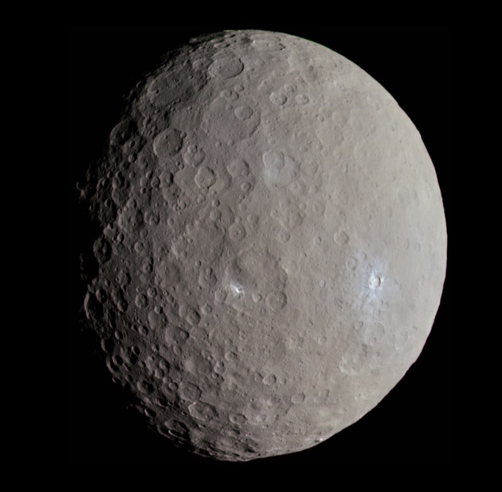
Gauss, then twenty-four, undertook the task. Using his own methods — including the minimisation of the sum of squared errors for the redundant observations — he computed the orbit and indicated where to look. In December 1801, Franz von Zach and Heinrich Olbers recovered Ceres close to Gauss’s prediction. The success made him famous across Europe.
Theoria Motus (1809) and the priority dispute
In Theoria Motus Corporum Coelestium in Sectionibus Conicis Solem Ambientium (1809), Gauss presented the method together with a deep justification, and stated that he had used it since 1795 — long before Legendre’s publication. This ignited one of the most famous priority disputes in the history of science. In Davis’s standard 1857 English translation, Gauss writes:
The modern assessment is usually balanced:
- Legendre was first to publish the method and to name it;
- Gauss was first to use it (though without publishing) and — more importantly — first to explain why the squares are the right choice.
Gauss’s original reasoning
Gauss asked the question Legendre had not: why the sum of squares? He took as his starting point a principle that astronomers already applied:
His genius lay in reversing the question: instead of “what is the best value for a given law of error?”, Gauss asked — which law of error $\varphi(\varepsilon)$ makes the arithmetic mean the best value? The answer forces the shape of the error distribution, and that shape turns out to be the normal distribution.
- Setup. Let $M_1,\dots,M_n$ be $n$ independent measurements of a quantity $\mu$; the error $\varepsilon_i = M_i - \mu$ has an unknown, symmetric density $\varphi(\varepsilon)$. The likelihood is $$ \Omega(\mu) = \varphi(M_1-\mu)\cdots\varphi(M_n-\mu). $$
- First-order condition. From $\frac{d}{d\mu}\log\Omega = 0$, writing $f := (\log\varphi)' = \varphi'/\varphi$: $$ \sum_{i=1}^n f(M_i-\hat\mu) = 0. $$
- Impose the postulate. Require $\hat\mu = \bar M$ for every sample. Then $\sum_i(M_i-\bar M)=0$, so the condition reads $\sum_i f(\varepsilon_i)=0$ whenever $\sum_i \varepsilon_i = 0$.
- This forces linearity. For the configuration $\varepsilon_1=(n-1)t,\ \varepsilon_2=\dots=\varepsilon_n=-t$ (which sums to zero) and odd $f$, one obtains $f((n-1)t)=(n-1)f(t)$ for all $t,n$ — hence $f(\varepsilon)=k\varepsilon$.
- Integrate. $(\log\varphi)'=k\varepsilon \Rightarrow \varphi(\varepsilon)=C\,e^{k\varepsilon^2/2}$.
- Density condition. For $\varphi$ to be an integrable density, $k<0$; writing $k=-2h^2$: $$ \boxed{\;\varphi(\varepsilon) = \frac{h}{\sqrt{\pi}}\,e^{-h^2\varepsilon^2}\;} $$ This is the normal distribution; $h$ is Gauss's *measure of precision* ($\textit{Genauigkeit}$). Hence its name — the Gaussian distribution.
The final step is immediate: since $\Omega \propto \exp(-h^2\sum\varepsilon_i^2)$, maximising the likelihood is equivalent to minimising the sum of squares $\sum\varepsilon_i^2$. This is least squares as maximum-likelihood estimation.
Part IV. Laplace: the probabilistic foundation

Gauss’s 1809 argument rested on the postulate of the mean — elegant, but arbitrary. An independent foundation came from Pierre-Simon Laplace. In 1810 he proved the central limit theorem: the sum of many small, independent influences is approximately normal.
This explained why a measurement error — being the sum of many tiny, independent disturbances — is in practice Gaussian. Laplace connected this with the method of least squares (Théorie analytique des probabilités, 1812), giving it a large-sample justification independent of Gauss’s postulate. This convergence of two routes is sometimes called the Gauss-Laplace synthesis; it secured the place of the normal distribution and of least squares throughout science. See the article on the central limit theorem.
Part V. Gauss again: the Gauss-Markov theorem (1823)
Gauss himself judged the 1809 argument unsatisfactory (it depended on the assumption of normality). In Theoria combinationis observationum erroribus minimis obnoxiae (1821–1823) he gave a wholly new justification requiring no particular law of error.
This was a more mature and more powerful argument. Gauss moved from “the mean is best, hence errors are normal, hence squares” to a purely variance-based argument: among reasonable (linear, unbiased) rules, least squares yields the least-dispersed estimates — irrespective of the shape of the error distribution. It is this result that makes least squares the foundation of classical econometrics, in which normality is seldom assumed yet least squares is trusted nonetheless.
Part VI. From measurement error to regression (nineteenth–twentieth centuries)
For most of the nineteenth century, least squares served astronomy and geodesy — estimating physical constants. The decisive turn towards a statistics of relationships came near the century’s end:
- Francis Galton (1822–1911), studying the heights of parents and children, observed “regression towards the mean” (1885) and coined the term regression. He moved the method from “errors” to relationships between variables.
- Karl Pearson (1857–1936) formalised the correlation coefficient (1896) and developed the regression apparatus.
- George Udny Yule (1871–1951) showed (1897) that multiple regression is simply least squares applied to several explanatory variables.
- Ronald A. Fisher (1890–1962) unified the theory: maximum likelihood, the analysis of variance, the properties of estimators. In his framework least squares is the maximum-likelihood estimator under normal errors — closing the circle Gauss had opened.
Thus a tool of astronomers became the foundation of econometrics: with the very calculus by which Gauss caught a planet, we now estimate the returns to education or the elasticity of demand.
Part VII. Matrix formulation of the model
Modern econometrics writes the linear model in matrix form, which renders the entire calculus compact and general. With $n$ observations and $k$ parameters,
$$ \mathbf{y} = \mathbf{X}\boldsymbol{\beta} + \boldsymbol{\varepsilon}, $$where $\mathbf{y}$ is the $n\times 1$ vector of the dependent variable, $\mathbf{X}$ the $n\times k$ matrix of regressors (the first column usually ones, for the intercept), $\boldsymbol{\beta}$ the $k\times 1$ vector of unknown parameters, and $\boldsymbol{\varepsilon}$ the $n\times 1$ vector of disturbances.
- A1. Linearity: $\mathbf{y} = \mathbf{X}\boldsymbol{\beta} + \boldsymbol{\varepsilon}$.
- A2. Full rank: $\operatorname{rank}(\mathbf{X}) = k$ (no perfect collinearity; $\mathbf{X}^\top\mathbf{X}$ invertible).
- A3. Exogeneity: $\mathbb{E}[\boldsymbol{\varepsilon}\mid\mathbf{X}] = \mathbf{0}$.
- A4. Sphericity: $\mathrm{Var}(\boldsymbol{\varepsilon}\mid\mathbf{X}) = \sigma^2\mathbf{I}_n$ (homoskedasticity and no autocorrelation).
- A5. Normality (optional, for exact finite-sample inference): $\boldsymbol{\varepsilon}\mid\mathbf{X}\sim\mathcal{N}(\mathbf{0},\sigma^2\mathbf{I}_n)$.
Assumptions A1–A4 are exactly the conditions of the Gauss-Markov theorem. Normality (A5) is not required for the optimality of least squares — it serves only for exact $t$ and $F$ tests in small samples.
Part VIII. Derivation of the estimator (matrix form)
We minimise the residual sum of squares written as an inner product:
$$ S(\boldsymbol{\beta}) = (\mathbf{y}-\mathbf{X}\boldsymbol{\beta})^\top(\mathbf{y}-\mathbf{X}\boldsymbol{\beta}) = \mathbf{y}^\top\mathbf{y} - 2\boldsymbol{\beta}^\top\mathbf{X}^\top\mathbf{y} + \boldsymbol{\beta}^\top\mathbf{X}^\top\mathbf{X}\boldsymbol{\beta}. $$- Gradient. Differentiating with respect to $\boldsymbol{\beta}$ (matrix calculus: $\partial(\mathbf{a}^\top\boldsymbol\beta)/\partial\boldsymbol\beta=\mathbf{a}$, $\partial(\boldsymbol\beta^\top\mathbf{A}\boldsymbol\beta)/\partial\boldsymbol\beta=2\mathbf{A}\boldsymbol\beta$): $$ \frac{\partial S}{\partial\boldsymbol\beta} = -2\mathbf{X}^\top\mathbf{y} + 2\mathbf{X}^\top\mathbf{X}\boldsymbol\beta. $$
- First-order condition. Setting this to zero gives the normal equations: $$ \mathbf{X}^\top\mathbf{X}\,\hat{\boldsymbol\beta} = \mathbf{X}^\top\mathbf{y}. $$
- Solution. By A2, $\mathbf{X}^\top\mathbf{X}$ is invertible, so $$ \boxed{\;\hat{\boldsymbol\beta} = (\mathbf{X}^\top\mathbf{X})^{-1}\mathbf{X}^\top\mathbf{y}\;} $$
- It is a minimum. The Hessian $2\mathbf{X}^\top\mathbf{X}$ is positive definite (full rank), so the critical point is the global minimum.
Part IX. Geometry: the hat matrix and orthogonal projection
The fitted values are $\hat{\mathbf{y}} = \mathbf{X}\hat{\boldsymbol\beta} = \mathbf{H}\mathbf{y}$, with $\mathbf{H} = \mathbf{X}(\mathbf{X}^\top\mathbf{X})^{-1}\mathbf{X}^\top$ the hat matrix — the orthogonal projection onto the column space of $\mathbf{X}$. The residuals are $\mathbf{e} = \mathbf{M}\mathbf{y}$ with $\mathbf{M} = \mathbf{I}-\mathbf{H}$, the annihilator matrix.
Both are symmetric and idempotent ($\mathbf{H}^2=\mathbf{H}$, $\mathbf{M}^2=\mathbf{M}$), and
$$ \mathbf{H}\mathbf{X}=\mathbf{X},\quad \mathbf{M}\mathbf{X}=\mathbf{0},\quad \operatorname{tr}(\mathbf{H})=k,\quad \operatorname{tr}(\mathbf{M})=n-k. $$Hence the orthogonality of residuals to the regressors: $\mathbf{X}^\top\mathbf{e}=\mathbf{0}$ — the same normal equation, now read geometrically. The residual vector is perpendicular to the column space of $\mathbf{X}$, and $\hat{\mathbf{y}}$ is the point of that space closest to $\mathbf{y}$.
Part X. Properties of the estimator
Substituting $\mathbf{y}=\mathbf{X}\boldsymbol\beta+\boldsymbol\varepsilon$ yields the key identity $\hat{\boldsymbol\beta} = \boldsymbol\beta + (\mathbf{X}^\top\mathbf{X})^{-1}\mathbf{X}^\top\boldsymbol\varepsilon$, from which:
- Unbiasedness: $\mathbb{E}[\hat{\boldsymbol\beta}\mid\mathbf{X}] = \boldsymbol\beta$ (by A3).
- Covariance: $\mathrm{Var}(\hat{\boldsymbol\beta}\mid\mathbf{X}) = \sigma^2(\mathbf{X}^\top\mathbf{X})^{-1}$ (by A4).
- Estimator of $\sigma^2$: $s^2 = \mathbf{e}^\top\mathbf{e}/(n-k)$ is unbiased ($k$ degrees of freedom are absorbed by the estimated parameters).
- Residuals as a function of the errors. Since $\mathbf{M}\mathbf{X}=\mathbf{0}$, substituting $\mathbf{y}=\mathbf{X}\boldsymbol\beta+\boldsymbol\varepsilon$ gives $\mathbf{e}=\mathbf{M}\mathbf{y}=\mathbf{M}\mathbf{X}\boldsymbol\beta+\mathbf{M}\boldsymbol\varepsilon=\mathbf{M}\boldsymbol\varepsilon$. The residuals do not depend on $\boldsymbol\beta$ — they are the filtered errors.
- Residual sum of squares. By the symmetry and idempotence of $\mathbf{M}$ ($\mathbf{M}^\top\mathbf{M}=\mathbf{M}^2=\mathbf{M}$): $$ \mathbf{e}^\top\mathbf{e}=\boldsymbol\varepsilon^\top\mathbf{M}^\top\mathbf{M}\boldsymbol\varepsilon=\boldsymbol\varepsilon^\top\mathbf{M}\boldsymbol\varepsilon. $$
- The trace trick. $\boldsymbol\varepsilon^\top\mathbf{M}\boldsymbol\varepsilon$ is a scalar, hence equal to its own trace; by the cyclic invariance of the trace, $\operatorname{tr}(\mathbf{M}\boldsymbol\varepsilon\boldsymbol\varepsilon^\top)$: $$ \mathbb{E}[\mathbf{e}^\top\mathbf{e}\mid\mathbf{X}]=\mathbb{E}\big[\operatorname{tr}(\mathbf{M}\boldsymbol\varepsilon\boldsymbol\varepsilon^\top)\big]=\operatorname{tr}\!\big(\mathbf{M}\,\mathbb{E}[\boldsymbol\varepsilon\boldsymbol\varepsilon^\top]\big)=\operatorname{tr}(\mathbf{M}\,\sigma^2\mathbf{I})=\sigma^2\operatorname{tr}(\mathbf{M}). $$
- Result. Since $\operatorname{tr}(\mathbf{M})=n-k$, we have $\mathbb{E}[\mathbf{e}^\top\mathbf{e}\mid\mathbf{X}]=\sigma^2(n-k)$, whence $$ \mathbb{E}[s^2\mid\mathbf{X}]=\frac{\mathbb{E}[\mathbf{e}^\top\mathbf{e}\mid\mathbf{X}]}{n-k}=\sigma^2. $$ The divisor $n-k$ — not $n$ — thus follows directly from the trace of the projection onto the residual space. Dividing by $n$ would bias the estimator downward by the factor $(n-k)/n$.
Part XI. The Gauss-Markov theorem — matrix proof
- Any linear estimator. Let $\tilde{\boldsymbol\beta} = \mathbf{C}\mathbf{y}$. Write $\mathbf{C} = (\mathbf{X}^\top\mathbf{X})^{-1}\mathbf{X}^\top + \mathbf{D}$.
- Unbiasedness. $\mathbb{E}[\tilde{\boldsymbol\beta}\mid\mathbf{X}]=\mathbf{C}\mathbf{X}\boldsymbol\beta$; unbiasedness for all $\boldsymbol\beta$ requires $\mathbf{C}\mathbf{X}=\mathbf{I}$, hence $\mathbf{D}\mathbf{X}=\mathbf{0}$.
- Covariance. Using $\mathbf{D}\mathbf{X}=\mathbf{0}$, the cross terms vanish and $\mathbf{C}\mathbf{C}^\top = (\mathbf{X}^\top\mathbf{X})^{-1} + \mathbf{D}\mathbf{D}^\top$.
- Conclusion. Therefore $$ \mathrm{Var}(\tilde{\boldsymbol\beta}\mid\mathbf{X}) = \sigma^2(\mathbf{X}^\top\mathbf{X})^{-1} + \sigma^2\mathbf{D}\mathbf{D}^\top, $$ and $\mathbf{D}\mathbf{D}^\top$ is positive semidefinite. Thus every other linear unbiased estimator has covariance no smaller than that of least squares, with equality only for $\mathbf{D}=\mathbf{0}$. This is BLUE.
Part XII. Distributions and inference (under normality)
Under A5, $\hat{\boldsymbol\beta}\sim\mathcal{N}\big(\boldsymbol\beta,\ \sigma^2(\mathbf{X}^\top\mathbf{X})^{-1}\big)$ and $(n-k)s^2/\sigma^2\sim\chi^2_{n-k}$. Replacing the unknown $\sigma^2$ by $s^2$ gives, for a single coefficient,
$$ \frac{\hat\beta_j-\beta_j}{\operatorname{SE}(\hat\beta_j)}\sim t_{n-k},\qquad \operatorname{SE}(\hat\beta_j)=s\sqrt{[(\mathbf{X}^\top\mathbf{X})^{-1}]_{jj}}, $$and, for $q$ joint linear restrictions, an $F_{q,\,n-k}$ statistic. This is the formal basis of hypothesis testing, the p-value and confidence intervals. Below we derive these distributions from first principles — from the single assumption that the disturbances are normal.
- Everything is linear in $\boldsymbol\varepsilon$. From the identities $\hat{\boldsymbol\beta}-\boldsymbol\beta=(\mathbf{X}^\top\mathbf{X})^{-1}\mathbf{X}^\top\boldsymbol\varepsilon$ and $\mathbf{e}=\mathbf{M}\boldsymbol\varepsilon$, both the estimator and the residuals are linear transformations of $\boldsymbol\varepsilon\sim\mathcal{N}(\mathbf{0},\sigma^2\mathbf{I})$. They are therefore jointly normal.
- (a) Independence of $\hat{\boldsymbol\beta}$ and $s^2$. Since $\mathbf{X}^\top\mathbf{H}=\mathbf{X}^\top$ (because $\mathbf{H}\mathbf{X}=\mathbf{X}$ and $\mathbf{H}$ is symmetric), $\hat{\boldsymbol\beta}-\boldsymbol\beta=(\mathbf{X}^\top\mathbf{X})^{-1}\mathbf{X}^\top\mathbf{H}\boldsymbol\varepsilon$ is a function of the component $\mathbf{H}\boldsymbol\varepsilon$. The residuals depend only on $\mathbf{M}\boldsymbol\varepsilon$. Their covariance $$ \mathrm{Cov}(\mathbf{H}\boldsymbol\varepsilon,\ \mathbf{M}\boldsymbol\varepsilon)=\mathbf{H}\,(\sigma^2\mathbf{I})\,\mathbf{M}^\top=\sigma^2\mathbf{H}\mathbf{M}=\mathbf{0}, $$ since $\mathbf{H}\mathbf{M}=\mathbf{0}$. For jointly normal vectors, zero covariance means independence, so $\hat{\boldsymbol\beta}$ is independent of $\mathbf{e}$, and hence of $s^2=\mathbf{e}^\top\mathbf{e}/(n-k)$.
- (b) Distribution of $s^2$. By the symmetry and idempotence of $\mathbf{M}$: $(n-k)s^2=\mathbf{e}^\top\mathbf{e}=\boldsymbol\varepsilon^\top\mathbf{M}^\top\mathbf{M}\boldsymbol\varepsilon=\boldsymbol\varepsilon^\top\mathbf{M}\boldsymbol\varepsilon$. Setting $\mathbf{z}=\boldsymbol\varepsilon/\sigma\sim\mathcal{N}(\mathbf{0},\mathbf{I})$, $$ \frac{(n-k)s^2}{\sigma^2}=\mathbf{z}^\top\mathbf{M}\mathbf{z}. $$ The matrix $\mathbf{M}$ — symmetric and idempotent — has eigenvalues $1$ (with multiplicity $\operatorname{tr}\mathbf{M}=n-k$) and $0$. In its eigenbasis $\mathbf{w}=\mathbf{Q}^\top\mathbf{z}\sim\mathcal{N}(\mathbf{0},\mathbf{I})$, so the quadratic form reduces to a sum of $n-k$ independent squared standard normals: $$ \mathbf{z}^\top\mathbf{M}\mathbf{z}=\sum_{i=1}^{n-k}w_i^2\sim\chi^2_{n-k}. $$
- (c) The $t$ statistic. For a single coefficient $\hat\beta_j\sim\mathcal{N}(\beta_j,\ \sigma^2 v_{jj})$, where $v_{jj}=[(\mathbf{X}^\top\mathbf{X})^{-1}]_{jj}$, so $Z=(\hat\beta_j-\beta_j)/(\sigma\sqrt{v_{jj}})\sim\mathcal{N}(0,1)$. Replacing the unknown $\sigma$ by $s$ and dividing by the square root of an independent $\chi^2$ over its degrees of freedom: $$ \frac{\hat\beta_j-\beta_j}{s\sqrt{v_{jj}}}=\frac{Z}{\sqrt{\dfrac{(n-k)s^2/\sigma^2}{n-k}}}=\frac{\mathcal{N}(0,1)}{\sqrt{\chi^2_{n-k}/(n-k)}}\sim t_{n-k}, $$ since numerator and denominator are independent by part (a). This is the definition of Student's $t$.
- (c) The $F$ statistic. Under $q$ restrictions $\mathbf{R}\boldsymbol\beta=\mathbf{r}$ and a true null, the vector $\mathbf{R}\hat{\boldsymbol\beta}-\mathbf{r}\sim\mathcal{N}\big(\mathbf{0},\ \sigma^2\mathbf{R}(\mathbf{X}^\top\mathbf{X})^{-1}\mathbf{R}^\top\big)$. The standardised quadratic form of this vector is a $\chi^2$ on $q$ degrees of freedom: $$ \frac{(\mathbf{R}\hat{\boldsymbol\beta}-\mathbf{r})^\top[\mathbf{R}(\mathbf{X}^\top\mathbf{X})^{-1}\mathbf{R}^\top]^{-1}(\mathbf{R}\hat{\boldsymbol\beta}-\mathbf{r})}{\sigma^2}\sim\chi^2_q. $$ The ratio of two independent $\chi^2$ variables, each divided by its own degrees of freedom, follows the $F$ distribution: $$ F=\frac{\chi^2_q/q}{\chi^2_{n-k}/(n-k)}\sim F_{q,\,n-k}, $$ with $\sigma^2$ cancelling between numerator and denominator — hence the final formula with $s^2$ in the denominator.
Part XIII. The Frisch-Waugh-Lovell theorem
One of the most important results on the interpretation of multiple regression (Frisch and Waugh 1933; Lovell 1963).
Partition the regressors as $\mathbf{X}=[\mathbf{X}_1\ \mathbf{X}_2]$. The OLS coefficient on $\mathbf{X}_2$ in the full regression is identical to the coefficient from regressing
the residuals of $\mathbf{y}$ on $\mathbf{X}_1$ against the residuals of $\mathbf{X}_2$ on $\mathbf{X}_1$.
In other words: the coefficient on a variable in a multiple regression is its effect after the influence of the remaining variables has been “partialled out” — the formal meaning of the phrase ceteris paribus.
- Normal equations of the full model. For $\mathbf{X}=[\mathbf{X}_1\ \mathbf{X}_2]$ and $\hat{\boldsymbol\beta}=[\hat{\boldsymbol\beta}_1;\ \hat{\boldsymbol\beta}_2]$, the system $\mathbf{X}^\top\mathbf{X}\hat{\boldsymbol\beta}=\mathbf{X}^\top\mathbf{y}$ splits into two blocks: $$ \mathbf{X}_1^\top\mathbf{X}_1\hat{\boldsymbol\beta}_1 + \mathbf{X}_1^\top\mathbf{X}_2\hat{\boldsymbol\beta}_2 = \mathbf{X}_1^\top\mathbf{y},\qquad \mathbf{X}_2^\top\mathbf{X}_1\hat{\boldsymbol\beta}_1 + \mathbf{X}_2^\top\mathbf{X}_2\hat{\boldsymbol\beta}_2 = \mathbf{X}_2^\top\mathbf{y}. $$
- Eliminate $\hat{\boldsymbol\beta}_1$. From the first block $\hat{\boldsymbol\beta}_1=(\mathbf{X}_1^\top\mathbf{X}_1)^{-1}\mathbf{X}_1^\top(\mathbf{y}-\mathbf{X}_2\hat{\boldsymbol\beta}_2)$. Substituting into the second, with the projection $\mathbf{P}_1=\mathbf{X}_1(\mathbf{X}_1^\top\mathbf{X}_1)^{-1}\mathbf{X}_1^\top$: $$ \mathbf{X}_2^\top\mathbf{P}_1(\mathbf{y}-\mathbf{X}_2\hat{\boldsymbol\beta}_2) + \mathbf{X}_2^\top\mathbf{X}_2\hat{\boldsymbol\beta}_2 = \mathbf{X}_2^\top\mathbf{y}. $$
- Collect terms. Rearranging and grouping in $\hat{\boldsymbol\beta}_2$, with $\mathbf{M}_1=\mathbf{I}-\mathbf{P}_1$ (the annihilator of $\mathbf{X}_1$): $$ \mathbf{X}_2^\top\mathbf{M}_1\mathbf{X}_2\,\hat{\boldsymbol\beta}_2 = \mathbf{X}_2^\top\mathbf{M}_1\mathbf{y}. $$
- Symmetry and idempotence. Since $\mathbf{M}_1=\mathbf{M}_1^\top=\mathbf{M}_1^2$, we have $\mathbf{X}_2^\top\mathbf{M}_1\mathbf{X}_2=(\mathbf{M}_1\mathbf{X}_2)^\top(\mathbf{M}_1\mathbf{X}_2)$ and $\mathbf{X}_2^\top\mathbf{M}_1\mathbf{y}=(\mathbf{M}_1\mathbf{X}_2)^\top(\mathbf{M}_1\mathbf{y})$. Hence $$ \boxed{\;\hat{\boldsymbol\beta}_2 = \big[(\mathbf{M}_1\mathbf{X}_2)^\top(\mathbf{M}_1\mathbf{X}_2)\big]^{-1}(\mathbf{M}_1\mathbf{X}_2)^\top(\mathbf{M}_1\mathbf{y})\;} $$ which is exactly the OLS estimator from regressing the **residuals** $\mathbf{M}_1\mathbf{y}$ (of $\mathbf{y}$ on $\mathbf{X}_1$) on the **residuals** $\mathbf{M}_1\mathbf{X}_2$ (of $\mathbf{X}_2$ on $\mathbf{X}_1$).
The theorem explains why coefficients of multiple regression are read as ceteris paribus effects, and it is a proof device in the theory of panel data and fixed-effects estimators.
Take $n=5$, two regressors and an intercept:
| $x_1$ | 1 | 2 | 3 | 4 | 5 |
|---|---|---|---|---|---|
| $x_2$ | 2 | 1 | 5 | 3 | 4 |
| $y$ | 3 | 2 | 6 | 5 | 7 |
The full regression of $y$ on $\{1, x_1, x_2\}$ gives the coefficient on $x_2$ equal to $\hat\beta_2 = \tfrac{27}{32} = 0.84375$.
Via FWL — first “clean” $y$ and $x_2$ of the influence of $\{1, x_1\}$ (take the residuals of each from a regression on a constant and $x_1$):
$$ \mathbf{M}_1\mathbf{y} = (0.6,\ -1.5,\ 1.4,\ -0.7,\ 0.2), \qquad \mathbf{M}_1\mathbf{x}_2 = (0.2,\ -1.4,\ 2.0,\ -0.6,\ -0.2). $$Regressing residuals on residuals (through the origin):
$$ \hat\beta_2 = \frac{(\mathbf{M}_1\mathbf{x}_2)^\top(\mathbf{M}_1\mathbf{y})}{(\mathbf{M}_1\mathbf{x}_2)^\top(\mathbf{M}_1\mathbf{x}_2)} = \frac{5.4}{6.4} = \frac{27}{32} = 0.84375. $$Identical — exactly as the theorem predicts.
Part XIV. Violations of the assumptions — a map
Each assumption A1–A5 can be broken; each breach has its own diagnosis and remedy. Details in the dedicated articles:
| Broken assumption | Effect | Diagnosis | Remedy |
|---|---|---|---|
| A1 linearity | bias | residual pattern | quadratic terms, logarithms |
| A2 full rank | none/instability | VIF | drop/combine variables, regularisation |
| A3 exogeneity | bias and inconsistency | subject-matter argument | instrumental variables, panel |
| A4 homoskedasticity | wrong SE | Breusch-Pagan | robust SE, WLS |
| A4 no autocorrelation | wrong SE | Breusch-Godfrey | HAC errors |
| A5 normality | small-sample tests | Q-Q, Shapiro | larger sample (CLT), bootstrap |
Part XV. Computational methods and extensions
In practice one does not invert $\mathbf{X}^\top\mathbf{X}$ explicitly — it is numerically unstable, since the condition number is squared: $\kappa(\mathbf{X}^\top\mathbf{X})=\kappa(\mathbf{X})^2$. Preferred are:
- QR decomposition: $\mathbf{X}=\mathbf{Q}\mathbf{R}$ (orthogonal-triangular), then $\mathbf{R}\hat{\boldsymbol\beta}=\mathbf{Q}^\top\mathbf{y}$ solved by back-substitution; the standard in R’s
lm()andlstsq. - Singular value decomposition: $\mathbf{X}=\mathbf{U}\boldsymbol\Sigma\mathbf{V}^\top$ — the most stable, handling even a (near-)rank-deficient $\mathbf{X}$; yields the Moore-Penrose pseudoinverse.
- Cholesky factorisation: $\mathbf{X}^\top\mathbf{X}=\mathbf{L}\mathbf{L}^\top$ — fast when conditioning is good.
- Gaussian elimination — the algorithm Gauss developed precisely to solve the normal equations by hand; still the basis of solving linear systems.
The principal statistical extensions:
- Weighted least squares (WLS): under known heteroskedasticity, minimise $\sum w_i\varepsilon_i^2$; $\hat{\boldsymbol\beta}=(\mathbf{X}^\top\mathbf{W}\mathbf{X})^{-1}\mathbf{X}^\top\mathbf{W}\mathbf{y}$.
- Generalised least squares (GLS): for any $\mathrm{Var}(\boldsymbol\varepsilon)=\sigma^2\boldsymbol\Omega$: $\hat{\boldsymbol\beta}=(\mathbf{X}^\top\boldsymbol\Omega^{-1}\mathbf{X})^{-1}\mathbf{X}^\top\boldsymbol\Omega^{-1}\mathbf{y}$ (Aitken).
- Instrumental variables / 2SLS: under endogeneity, $\hat{\boldsymbol\beta}_{IV}=(\mathbf{Z}^\top\mathbf{X})^{-1}\mathbf{Z}^\top\mathbf{y}$ — see IV.
- Ridge and lasso: add a penalty on coefficient size; ridge: $\hat{\boldsymbol\beta}=(\mathbf{X}^\top\mathbf{X}+\lambda\mathbf{I})^{-1}\mathbf{X}^\top\mathbf{y}$ — stabilises under collinearity and in high dimension.
- Nonlinear least squares (NLS): minimise $\sum(y_i-f(\mathbf{x}_i,\boldsymbol\beta))^2$ for nonlinear $f$, by iterative methods (Gauss-Newton).
Part XVI. Connections to other methods of estimation
- Maximum likelihood: under normal errors, ML coincides exactly with least squares (Part III).
- Bayes: with a flat prior, the posterior for $\boldsymbol\beta$ is centred at $\hat{\boldsymbol\beta}_{\text{OLS}}$; a conjugate normal prior yields ridge regression.
- Method of moments: the condition $\mathbb{E}[\mathbf{X}^\top\boldsymbol\varepsilon]=\mathbf{0}$, in sample form $\mathbf{X}^\top\mathbf{e}=\mathbf{0}$, is again the normal equations.
Part XVII. A worked example: regression step by step
The entire theory reduces to a handful of arithmetic operations. Let us carry them out by hand on a small dataset ($n=5$, one regressor and an intercept), so as to see exactly where every number reported by a statistical package comes from.
| $i$ | $x_i$ | $y_i$ |
|---|---|---|
| 1 | 1 | 2 |
| 2 | 2 | 4 |
| 3 | 3 | 5 |
| 4 | 4 | 4 |
| 5 | 5 | 5 |
Model: $y_i = \beta_0 + \beta_1 x_i + \varepsilon_i$. Means: $\bar x = 3$, $\bar y = 4$.
Step 1. Sums and matrices
The design matrix $\mathbf{X}$ has ones in its first column (the intercept) and the values $x_i$ in the second. Hence
$$ \mathbf{X}^\top\mathbf{X} = \begin{bmatrix} n & \sum x_i \\ \sum x_i & \sum x_i^2 \end{bmatrix} = \begin{bmatrix} 5 & 15 \\ 15 & 55 \end{bmatrix}, \qquad \mathbf{X}^\top\mathbf{y} = \begin{bmatrix} \sum y_i \\ \sum x_i y_i \end{bmatrix} = \begin{bmatrix} 20 \\ 66 \end{bmatrix}. $$The determinant is $\det(\mathbf{X}^\top\mathbf{X}) = 5\cdot 55 - 15^2 = 275 - 225 = 50$, so
$$ (\mathbf{X}^\top\mathbf{X})^{-1} = \frac{1}{50}\begin{bmatrix} 55 & -15 \\ -15 & 5 \end{bmatrix} = \begin{bmatrix} 1.1 & -0.3 \\ -0.3 & 0.1 \end{bmatrix}. $$Step 2. The estimator
$$ \hat{\boldsymbol\beta} = (\mathbf{X}^\top\mathbf{X})^{-1}\mathbf{X}^\top\mathbf{y} = \begin{bmatrix} 1.1 & -0.3 \\ -0.3 & 0.1 \end{bmatrix}\begin{bmatrix} 20 \\ 66 \end{bmatrix} = \begin{bmatrix} 22 - 19.8 \\ -6 + 6.6 \end{bmatrix} = \begin{bmatrix} 2.2 \\ 0.6 \end{bmatrix}. $$The scalar formulae for simple regression give the same result: with $S_{xx} = \sum(x_i-\bar x)^2 = 10$ and $S_{xy} = \sum(x_i-\bar x)(y_i-\bar y) = 6$,
$$ \hat\beta_1 = \frac{S_{xy}}{S_{xx}} = \frac{6}{10} = 0.6, \qquad \hat\beta_0 = \bar y - \hat\beta_1\bar x = 4 - 0.6\cdot 3 = 2.2. $$The fitted line: $\hat y = 2.2 + 0.6\,x$.
Step 3. Fitted values and residuals
| $i$ | $x_i$ | $y_i$ | $\hat y_i = 2.2+0.6x_i$ | $e_i = y_i-\hat y_i$ | $e_i^2$ |
|---|---|---|---|---|---|
| 1 | 1 | 2 | 2.8 | $-0.8$ | 0.64 |
| 2 | 2 | 4 | 3.4 | $0.6$ | 0.36 |
| 3 | 3 | 5 | 4.0 | $1.0$ | 1.00 |
| 4 | 4 | 4 | 4.6 | $-0.6$ | 0.36 |
| 5 | 5 | 5 | 5.2 | $-0.2$ | 0.04 |
| sum | $0.0$ | 2.40 |
The residuals sum to zero ($\sum e_i = 0$) — a direct consequence of the normal equations in the presence of an intercept. The residual sum of squares is $\text{RSS} = \mathbf{e}^\top\mathbf{e} = 2.40$.
Step 4. Residual variance and standard errors
With $n=5$, $k=2$, hence $n-k=3$ degrees of freedom:
$$ s^2 = \frac{\text{RSS}}{n-k} = \frac{2.40}{3} = 0.80. $$The estimated covariance matrix is $\widehat{\mathrm{Var}}(\hat{\boldsymbol\beta}) = s^2(\mathbf{X}^\top\mathbf{X})^{-1}$, whose diagonal yields the standard errors:
$$ \operatorname{SE}(\hat\beta_0) = \sqrt{0.80\cdot 1.1} = \sqrt{0.88} \approx 0.938, \qquad \operatorname{SE}(\hat\beta_1) = \sqrt{0.80\cdot 0.1} = \sqrt{0.08} \approx 0.283. $$Step 5. The $t$ statistics and significance
Under the null hypothesis $\beta_j = 0$:
$$ t_0 = \frac{2.2}{0.938} \approx 2.345, \qquad t_1 = \frac{0.6}{0.283} \approx 2.121. $$The critical value of $t$ for $3$ degrees of freedom at the $0.05$ level (two-sided) is $3.182$. Both statistics fall below it, so with such a small sample we fail to reject the hypothesis of zero coefficients at the 5% level — despite the apparent fit. This neatly illustrates how little information $n=5$ carries. See hypothesis testing and the p-value.
Step 6. Goodness of fit
The total sum of squares is $\text{TSS} = \sum(y_i-\bar y)^2 = 4+0+1+0+1 = 6$. Therefore
$$ R^2 = 1 - \frac{\text{RSS}}{\text{TSS}} = 1 - \frac{2.4}{6} = 0.60, $$the adjusted $\bar R^2 = 1 - (1-R^2)\dfrac{n-1}{n-k} = 1 - 0.4\cdot\dfrac{4}{3} \approx 0.467$, and the statistic
$$ F = \frac{(\text{TSS}-\text{RSS})/(k-1)}{\text{RSS}/(n-k)} = \frac{3.6/1}{2.4/3} = 4.5 = t_1^2, $$confirming the identity $F = t^2$ for a single regressor. The model explains 60% of the variation in $y$.
Part XVIII. A confidence interval for E[y₀] versus a prediction interval
Having fitted the model, at a point $\mathbf{x}_0$ we may ask two distinct questions. First: where does the conditional mean $\mathbb{E}[y\mid\mathbf{x}_0]=\mathbf{x}_0^\top\boldsymbol\beta$ lie? Second: what value will a new, single observation $y_0=\mathbf{x}_0^\top\boldsymbol\beta+\varepsilon_0$ take? Both share the same point estimate $\hat y_0=\mathbf{x}_0^\top\hat{\boldsymbol\beta}$, but carry different uncertainty — and that is the origin of the distinction between a confidence interval and a prediction interval.
- A common estimator. $\hat y_0=\mathbf{x}_0^\top\hat{\boldsymbol\beta}$ is an unbiased estimator of the mean $\mathbf{x}_0^\top\boldsymbol\beta$, since $\mathbb{E}[\hat{\boldsymbol\beta}\mid\mathbf{X}]=\boldsymbol\beta$.
- Variance of the conditional mean. The uncertainty comes only from estimating $\hat{\boldsymbol\beta}$: $$ \mathrm{Var}(\hat y_0\mid\mathbf{X})=\mathbf{x}_0^\top\mathrm{Var}(\hat{\boldsymbol\beta}\mid\mathbf{X})\mathbf{x}_0=\sigma^2\,\mathbf{x}_0^\top(\mathbf{X}^\top\mathbf{X})^{-1}\mathbf{x}_0. $$
- Prediction error for a new observation. A new observation $y_0=\mathbf{x}_0^\top\boldsymbol\beta+\varepsilon_0$ carries an additional, independent term $\varepsilon_0$ of variance $\sigma^2$. The prediction error decomposes as $y_0-\hat y_0=(\mathbf{x}_0^\top\boldsymbol\beta-\mathbf{x}_0^\top\hat{\boldsymbol\beta})+\varepsilon_0$; the two terms are independent (since $\varepsilon_0$ belongs to a future observation, absent from the sample), so the variances add: $$ \mathrm{Var}(y_0-\hat y_0\mid\mathbf{X})=\sigma^2\,\mathbf{x}_0^\top(\mathbf{X}^\top\mathbf{X})^{-1}\mathbf{x}_0+\sigma^2=\sigma^2\big(1+\mathbf{x}_0^\top(\mathbf{X}^\top\mathbf{X})^{-1}\mathbf{x}_0\big). $$ The extra "1" is the irreducible noise of a single observation — it persists even in an infinite sample, where $\hat{\boldsymbol\beta}\to\boldsymbol\beta$.
Replacing the unknown $\sigma^2$ by $s^2$ and using the $t_{n-k}$ distribution gives two intervals (at confidence level $1-\alpha$):
$$ \underbrace{\hat y_0\pm t_{n-k,\,\alpha/2}\;s\sqrt{\mathbf{x}_0^\top(\mathbf{X}^\top\mathbf{X})^{-1}\mathbf{x}_0}}_{\text{confidence interval for }\mathbb{E}[y_0]},\qquad \underbrace{\hat y_0\pm t_{n-k,\,\alpha/2}\;s\sqrt{1+\mathbf{x}_0^\top(\mathbf{X}^\top\mathbf{X})^{-1}\mathbf{x}_0}}_{\text{prediction interval for a new }y_0}. $$Take the model of Part XVII: $\hat{\boldsymbol\beta}=(2.2;\ 0.6)$, $s^2=0.8$, $(\mathbf{X}^\top\mathbf{X})^{-1}=\begin{bmatrix}1.1 & -0.3\\ -0.3 & 0.1\end{bmatrix}$, $n-k=3$, $t_{3;\,0.025}=3.182$. At the centre of the data $\mathbf{x}_0=(1,\ 3)$:
$$ \hat y_0=2.2+0.6\cdot 3=4.0,\qquad \mathbf{x}_0^\top(\mathbf{X}^\top\mathbf{X})^{-1}\mathbf{x}_0=\tfrac{1}{5}=0.2. $$The leverage $\mathbf{x}_0^\top(\mathbf{X}^\top\mathbf{X})^{-1}\mathbf{x}_0=0.2$ is the smallest possible here (the centre of the sample — the most reliable prediction).
- Confidence interval for $\mathbb{E}[y_0]$: $\operatorname{SE}=\sqrt{0.8\cdot 0.2}=\sqrt{0.16}=0.4$, so $4.0\pm 3.182\cdot 0.4=4.0\pm 1.273$, that is $[2.727;\ 5.273]$.
- Prediction interval for a new $y_0$: $\operatorname{SE}=\sqrt{0.8\cdot 1.2}=\sqrt{0.96}\approx 0.980$, so $4.0\pm 3.182\cdot 0.980=4.0\pm 3.118$, that is $[0.882;\ 7.118]$.
The prediction interval is markedly wider ($\pm 3.118$ against $\pm 1.273$) — it must cover not only the uncertainty about the location of the line, but also the random scatter of the observation itself. The gap does not vanish with the sample: as $n\to\infty$, the confidence interval shrinks to a point, while the prediction interval shrinks only to width $\pm t\cdot\sigma$.
Part XIX. The decomposition of variance: R², adjusted R² and the ANOVA table
How well does the model explain the variation in the data? The answer comes from splitting the total variation of $\mathbf{y}$ into a part explained by the regression and a residual part — the foundation of the analysis of variance (ANOVA) and of the coefficient of determination $R^2$. The three sums of squares (for a model with an intercept; $\bar y$ is the mean of $y$):
$$ \underbrace{\textstyle\sum_i (y_i-\bar y)^2}_{\text{TSS — total}}, \qquad \underbrace{\textstyle\sum_i (\hat y_i-\bar y)^2}_{\text{ESS — explained}}, \qquad \underbrace{\textstyle\sum_i (y_i-\hat y_i)^2}_{\text{RSS — residual}}. $$- Decompose the deviation. For each observation $y_i-\bar y=(\hat y_i-\bar y)+(y_i-\hat y_i)=(\hat y_i-\bar y)+e_i$. Squaring and summing over $i$: $$ \sum_i(y_i-\bar y)^2=\sum_i(\hat y_i-\bar y)^2+\sum_i e_i^2+2\sum_i(\hat y_i-\bar y)e_i. $$
- The cross term vanishes. $\sum_i(\hat y_i-\bar y)e_i=\sum_i\hat y_i e_i-\bar y\sum_i e_i$. By the normal equations the residuals are orthogonal to the regressors, $\mathbf{X}^\top\mathbf{e}=\mathbf{0}$; in particular the column of ones gives $\sum_i e_i=0$, and a combination of columns gives $\hat{\mathbf{y}}^\top\mathbf{e}=\hat{\boldsymbol\beta}^\top\mathbf{X}^\top\mathbf{e}=0$. Both terms are zero.
- Conclusion. $\text{TSS}=\text{ESS}+\text{RSS}$. Step 2 requires an intercept in the model — without it $\sum_i e_i\neq 0$ and the identity breaks down.
Hence the coefficient of determination:
$$ R^2=\frac{\text{ESS}}{\text{TSS}}=1-\frac{\text{RSS}}{\text{TSS}}\in[0,1], $$read as the share of the variation in $y$ explained by the model. Equivalently, $R^2$ is the square of the correlation coefficient between $y_i$ and $\hat y_i$.
The difficulty is that $R^2$ never decreases when a regressor is added (each new column can only lower the RSS). To penalise an excess of parameters one uses the adjusted $R^2$:
$$ \bar R^2=1-\frac{\text{RSS}/(n-k)}{\text{TSS}/(n-1)}=1-(1-R^2)\frac{n-1}{n-k}, $$which rises only when a new regressor improves the fit by more than chance alone would; $\bar R^2$ may be negative. The same sums of squares arrange themselves into an ANOVA table, from which the $F$ statistic for the joint significance of the regression follows directly:
| Source | Sum of squares | df | Mean square | $F$ |
|---|---|---|---|---|
| Regression | ESS | $k-1$ | $\text{ESS}/(k-1)$ | $\dfrac{\text{ESS}/(k-1)}{\text{RSS}/(n-k)}$ |
| Residual | RSS | $n-k$ | $\text{RSS}/(n-k)=s^2$ | |
| Total | TSS | $n-1$ |
For the data of Part XVII ($\hat y=2.2+0.6x$, $\bar y=4$):
$$ \text{TSS}=6,\qquad \text{ESS}=\sum_i(\hat y_i-4)^2=1.44+0.36+0+0.36+1.44=3.6,\qquad \text{RSS}=2.4, $$so $\text{ESS}+\text{RSS}=3.6+2.4=6=\text{TSS}$ — the identity holds. Therefore
$$ R^2=\frac{3.6}{6}=0.60,\qquad \bar R^2=1-0.4\cdot\frac{4}{3}=\frac{7}{15}\approx0.467. $$The ANOVA table for this fit:
| Source | SS | df | MS | $F$ |
|---|---|---|---|---|
| Regression | 3.6 | 1 | 3.6 | 4.5 |
| Residual | 2.4 | 3 | 0.8 | |
| Total | 6.0 | 4 |
The statistic $F=3.6/0.8=4.5$ — exactly $t_1^2=2.121^2$ from Part XVII (for a single regressor $F=t^2$). The model explains 60% of the variation in $y$.
Part XX. Multiple regression and omitted-variable bias — a worked example
Part XIII showed how the FWL theorem recovers a coefficient cleaned of the influence of the other variables. Here we compute the other side of the coin: what happens when a relevant variable is omitted. We use the same data as in Part XIII:
| $x_1$ | 1 | 2 | 3 | 4 | 5 |
|---|---|---|---|---|---|
| $x_2$ | 2 | 1 | 5 | 3 | 4 |
| $y$ | 3 | 2 | 6 | 5 | 7 |
The full regression of $y$ on $\{1,x_1,x_2\}$ — the solution of the normal equations $\hat{\boldsymbol\beta}=(\mathbf{X}^\top\mathbf{X})^{-1}\mathbf{X}^\top\mathbf{y}$ (exactly, in fractions):
$$ \hat\beta_0=\tfrac{23}{80}=0.2875,\qquad \hat\beta_1=\tfrac{19}{32}=0.59375,\qquad \hat\beta_2=\tfrac{27}{32}=0.84375. $$The short regression omitting $x_2$ (only $y$ on $\{1,x_1\}$):
$$ \tilde\beta_0=\tfrac{13}{10}=1.3,\qquad \tilde\beta_1=\tfrac{11}{10}=1.1. $$The coefficient on $x_1$ has jumped from $0.594$ to $1.1$ — nearly doubling. This is omitted-variable bias: the short coefficient attributes to $x_1$ part of the effect of $x_2$ as well, because the two variables are correlated.
- Auxiliary regression. Let $\delta$ be the slope from regressing the omitted variable on the retained regressors — here $x_2$ on $\{1,x_1\}$ — that is $\delta=S_{x_1x_2}/S_{x_1x_1}$.
- Sample identity. From the partitioned solution of the normal equations (the same algebra as in the FWL proof, Part XIII) follows the exact identity: $$ \tilde\beta_1=\hat\beta_1+\hat\beta_2\,\delta. $$ The short coefficient collects the own effect of $x_1$ (namely $\hat\beta_1$) augmented by the effect of $x_2$ (namely $\hat\beta_2$) "passed through" the correlation of $x_2$ with $x_1$ (namely $\delta$).
- Conclusion. The bias vanishes exactly when $\hat\beta_2=0$ (the omitted variable is irrelevant) or $\delta=0$ (the omitted variable is uncorrelated with the retained ones). This is the sample counterpart of [the exogeneity assumption](/en/ekonometria/zalozenia-kmnk/) A3.
Regressing $x_2$ on $\{1,x_1\}$ gives $\delta=S_{x_1x_2}/S_{x_1x_1}=6/10=0.6$ (since $\bar x_1=\bar x_2=3$, $S_{x_1x_2}=6$, $S_{x_1x_1}=10$). Then
$$ \hat\beta_1+\hat\beta_2\,\delta=\frac{19}{32}+\frac{27}{32}\cdot\frac{3}{5}=\frac{19}{32}+\frac{81}{160}=\frac{95+81}{160}=\frac{176}{160}=\frac{11}{10}=1.1=\tilde\beta_1. $$Exactly the coefficient from the short regression. For comparison of residuals: the full model has $\text{RSS}=87/160\approx0.544$, the short model $\text{RSS}=5.1$ — omitting $x_2$ worsens the fit several-fold and distorts the estimate of $x_1$ at the same time.
Appendix A. Summary of key formulae
| Quantity | Formula |
|---|---|
| Estimator | $\hat{\boldsymbol\beta}=(\mathbf{X}^\top\mathbf{X})^{-1}\mathbf{X}^\top\mathbf{y}$ |
| Fitted values | $\hat{\mathbf{y}}=\mathbf{H}\mathbf{y}$, $\mathbf{H}=\mathbf{X}(\mathbf{X}^\top\mathbf{X})^{-1}\mathbf{X}^\top$ |
| Residuals | $\mathbf{e}=\mathbf{M}\mathbf{y}$, $\mathbf{M}=\mathbf{I}-\mathbf{H}$ |
| Covariance | $\mathrm{Var}(\hat{\boldsymbol\beta})=\sigma^2(\mathbf{X}^\top\mathbf{X})^{-1}$ |
| Estimator of $\sigma^2$ | $s^2=\mathbf{e}^\top\mathbf{e}/(n-k)$ |
| $t$ statistic | $(\hat\beta_j-\beta_j)/\operatorname{SE}(\hat\beta_j)\sim t_{n-k}$ |
| $R^2$ | $1-\mathbf{e}^\top\mathbf{e}/\sum(y_i-\bar y)^2$ |
| Adjusted $R^2$ | $1-(1-R^2)\dfrac{n-1}{n-k}$ |
| $F$ statistic (ANOVA) | $\dfrac{\text{ESS}/(k-1)}{\text{RSS}/(n-k)}\sim F_{k-1,\,n-k}$ |
Appendix B. Notation
| Symbol | Meaning |
|---|---|
| $n,\ k$ | number of observations, number of parameters |
| $\mathbf{y},\ \mathbf{X},\ \boldsymbol\beta,\ \boldsymbol\varepsilon$ | vector of observations, regressor matrix, parameters, errors |
| $\hat{\boldsymbol\beta},\ \mathbf{e},\ \hat{\mathbf{y}}$ | estimator, residuals, fitted values |
| $\mathbf{H},\ \mathbf{M}$ | hat matrix, annihilator matrix |
| $\sigma^2,\ s^2$ | error variance and its estimator |
Appendix C. Biographical sketches
Brief notes on the figures whose work converged into the method of least squares and regression.
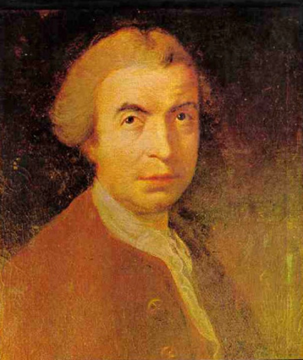
Adrien-Marie Legendre (1752–1833) — French mathematician, author of foundational works in number theory (Essai sur la théorie des nombres), elliptic functions and geometry (his Éléments de géométrie displaced Euclid in schools for a century). He was the first to publish the method of least squares (1805) and to name it. Late in life he lost his government pension after refusing to back the authorities’ candidate in an Institute vote, and died in poverty. The only surviving likeness of him is Boilly’s caricature.
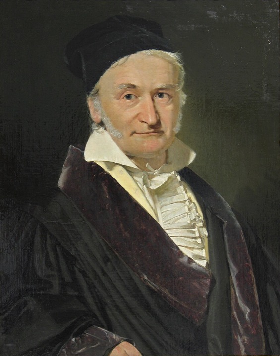
Carl Friedrich Gauss (1777–1855) — German mathematician, astronomer and physicist, called princeps mathematicorum, the “Prince of Mathematicians.” Born to a poor family in Brunswick, his gifts were recognised in childhood. In the Disquisitiones Arithmeticae (1801) he built modern number theory; he computed the orbit of Ceres; he proved the fundamental theorem of algebra (doctoral dissertation, 1799); and he advanced geodesy, magnetism and electrostatics (the unit of magnetic induction bears his name). For least squares the key works are Theoria Motus (1809) and Theoria combinationis (1821–1823).
Pierre-Simon de Laplace (1749–1827) — French mathematician and astronomer, creator of celestial mechanics (Traité de mécanique céleste) and of modern probability theory (Théorie analytique des probabilités, 1812). His central limit theorem explained why measurement errors tend to be normal, and tied least squares to the calculus of probability. He navigated the Revolution, the Empire and the Restoration while retaining influential scientific posts.
Ruđer Josip Bošković (1711–1787) — a scholar from Dubrovnik, a Jesuit, astronomer and physicist active in Italy. He proposed (1755–1760) the criterion closest in spirit to least squares: minimising the sum of absolute deviations subject to the signed deviations summing to zero — today’s $L_1$ regression, to which statistics returned only in the twentieth century.
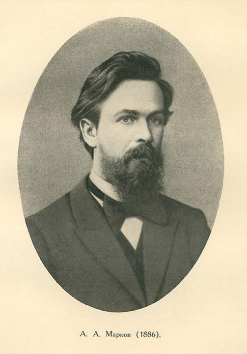
Andrey Markov (1856–1922) — Russian mathematician, a student of Chebyshev, and the founder of the theory of Markov chains. His name entered the Gauss-Markov theorem through later textbooks, although Gauss already had the result in 1823.
Francis Galton (1822–1911) — British polymath, a cousin of Darwin, and a student of heredity. He introduced the notion of regression (“reversion to the mean”) and of correlation, transferring the method from measurement errors to relationships between variables. (He was also a proponent of eugenics — an idea now rejected.)
Karl Pearson (1857–1936) — British mathematician and statistician, who formalised the correlation coefficient, the $\chi^2$ test and much of the apparatus of mathematical statistics; founder of the first chair of statistics (University College London) and of the journal Biometrika.
Ronald Aylmer Fisher (1890–1962) — British statistician and geneticist, one of the founders of modern statistics. He introduced maximum likelihood, the analysis of variance, the design of experiments and the notion of statistical significance, casting least squares as the maximum-likelihood estimator under normal errors.
Appendix D. The original texts and sources
A register of the primary works in which the method took shape, with the location of the key passages and the standard translations. The quotations in Parts II and III are drawn directly from these editions.
Legendre (1805). A. M. Legendre, Nouvelles méthodes pour la détermination des orbites des comètes, Paris: Firmin Didot, 1805. The first publication of the method appears in the appendix Sur la méthode des moindres carrés (pp. 72–80). It is the source of the famous sentence "…rendre minimum la somme des carrés des erreurs" (Part II).
Gauss (1809). C. F. Gauss, Theoria Motus Corporum Coelestium in Sectionibus Conicis Solem Ambientium, Hamburg: Perthes & Besser, 1809. The Latin original; the treatment of least squares occupies Book II, Section 3, articles 175–186. The standard English translation is C. H. Davis, Theory of the Motion of the Heavenly Bodies Moving about the Sun in Conic Sections, Boston: Little, Brown, 1857 — the source of the priority statement (Part III).
Gauss (1821–1823). C. F. Gauss, Theoria combinationis observationum erroribus minimis obnoxiae, Göttingen (Pars prior 1821, Pars posterior 1823) — the mature variance-based justification (the Gauss-Markov theorem). Annotated English translation: G. W. Stewart, Theory of the Combination of Observations Least Subject to Errors, SIAM, 1995.
Laplace (1812). P. S. Laplace, Théorie analytique des probabilités, Paris: Courcier, 1812 — the probabilistic treatment of error and the central limit theorem.
Translations and scholarship. English translations of many historical works (Legendre, Laplace and others) have been made available by Richard J. Pulskamp (probabilityandfinance.com). The classic historical account is S. M. Stigler, The History of Statistics: The Measurement of Uncertainty before 1900, Harvard University Press, 1986.
Appendix E. Bibliography and further reading
Modern treatments and classic source papers, complementing the primary texts of Appendix D. For the full history of the method, Stigler (1986), already cited above, remains indispensable.
Modern textbooks of econometrics and statistics.
- W. H. Greene, Econometric Analysis, Pearson, 8th ed., 2018 — the encyclopaedic academic standard; a complete treatment of the matrix linear model, the Gauss-Markov theorem, FWL and the extensions.
- J. M. Wooldridge, Introductory Econometrics: A Modern Approach, Cengage, 7th ed., 2019 — the most popular introduction; and his Econometric Analysis of Cross Section and Panel Data, MIT Press, 2nd ed., 2010 (advanced level).
- F. Hayashi, Econometrics, Princeton University Press, 2000 — a rigorous, method-of-moments-based treatment of least squares and GMM.
- R. Davidson, J. G. MacKinnon, Econometric Theory and Methods, Oxford University Press, 2004 — a strong emphasis on the geometry of projections and the FWL theorem.
- C. R. Rao, Linear Statistical Inference and Its Applications, Wiley, 2nd ed., 1973 — a classic of linear estimation theory.
- H. Theil, Principles of Econometrics, Wiley, 1971 — a historical reference point of modern econometrics.
Classic papers on the method and its history.
- R. Frisch, F. V. Waugh, “Partial Time Regressions as Compared with Individual Trends”, Econometrica 1(4), 1933, pp. 387–401 — the source of the FWL theorem.
- M. C. Lovell, “Seasonal Adjustment of Economic Time Series and Multiple Regression Analysis”, Journal of the American Statistical Association 58(304), 1963, pp. 993–1010 — the generalisation and the name of the theorem.
- A. C. Aitken, “On Least Squares and Linear Combination of Observations”, Proceedings of the Royal Society of Edinburgh 55, 1935, pp. 42–48 — generalised least squares (GLS).
- R. L. Plackett, “The Discovery of the Method of Least Squares”, Biometrika 59(2), 1972, pp. 239–251 — a detailed reconstruction of the priority dispute.
- S. M. Stigler, “Gauss and the Invention of Least Squares”, The Annals of Statistics 9(3), 1981, pp. 465–474 — an analysis of Gauss’s 1809 priority claim.
Chronology
| Year | Event |
|---|---|
| 1722 | Cotes — weighted mean of observations (posthumous) |
| 1736–44 | Lapland and Peru expeditions — the figure of the Earth |
| ~1750 | Tobias Mayer — method of averages (lunar libration) |
| 1755–60 | Bošković — minimising the sum of absolute deviations ($L_1$) |
| 1795 | Gauss begins (by his own account) using least squares |
| 1801 | Piazzi discovers Ceres; Gauss computes the orbit; the planet is recovered |
| 1805 | Legendre — first publication of the method of least squares |
| 1808 | Robert Adrain — independent derivation of the law of error |
| 1809 | Gauss, Theoria Motus — derivation from the postulate of the mean |
| 1810 | Laplace — the central limit theorem |
| 1823 | Gauss, Theoria combinationis — the Gauss-Markov theorem |
| 1885 | Galton — “regression”; the method applied to relationships |
| 1896 | Pearson — the correlation coefficient |
| 1922 | Fisher — maximum likelihood |
Legacy
From a single astronomical problem grew a tool underlying linear regression and the whole of econometrics, estimation theory, machine learning (the minimisation of squared error), and numerical linear algebra (Gaussian elimination, the QR and SVD decompositions). And the distribution Gauss derived “in passing,” while justifying his method, bears his name and is the most important distribution in all of statistics — in part through the central limit theorem.
Related: Ordinary Least Squares — a step-by-step derivation · The classical (OLS) assumptions
- C. F. Gauss, Theoria Motus Corporum Coelestium in Sectionibus Conicis Solem Ambientium (1809); trans. C. H. Davis, Theory of the Motion of the Heavenly Bodies (1857), arts. 175–186
- C. F. Gauss, Theoria combinationis observationum erroribus minimis obnoxiae (1821–1823)
- A. M. Legendre, Nouvelles méthodes pour la détermination des orbites des comètes (1805), appendix Sur la méthode des moindres carrés
- P. S. Laplace, Théorie analytique des probabilités (1812)
- S. M. Stigler, The History of Statistics: The Measurement of Uncertainty before 1900 (1986)